MATH5714 Linear Regression, Robustness and Smoothing
University of Leeds, Semester 1, 2025/26
Preface
The MATH5714M module includes all the material from MATH3714 (Linear Regression and Robustness), plus additional material on smoothing.
The level 3 component covers linear regression and its extensions. In simple linear regression, we fit a line through data points \((x_1, y_1), \ldots, (x_n, y_n) \in\mathbb{R}^2\) using the model \[\begin{equation*} y_i = \alpha + \beta x_i + \varepsilon_i \end{equation*}\] for all \(i \in \{1, 2, \ldots, n\}\), where the aim is to find values for the intercept \(\alpha\) and the slope \(\beta\) such that the fitted line is as close as possible to the data points.
However, linear models are not always appropriate. Figure 0.1 illustrates an example where a straight line model would be inadequate. For such data, we need more flexible methods that can capture non-linear patterns.
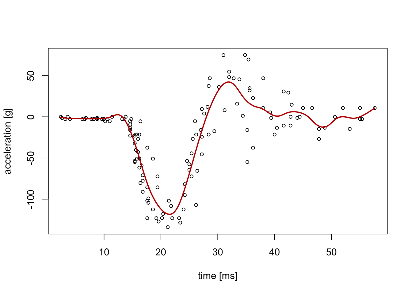
Figure 0.1: An illustration of a dataset where a linear (straight line) model is not appropriate. The data represents a series of measurements of head acceleration in a simulated motorcycle accident, used to test crash helmets (the mcycle dataset from the MASS R package).
The level 5 component introduces techniques for fitting smooth curves through data—methods collectively known as smoothing. Unlike linear regression, which imposes a straight line on all the data, smoothing methods work locally: they estimate the relationship at different points using nearby observations, then blend these local estimates together to create a smooth curve. The red curve in Figure 0.1 shows such a smoothed fit, which captures the complex pattern in the data without assuming any particular functional form.
We will approach these smoothing methods gradually. We begin with the simpler problem of “kernel density estimation”: given a sample from an unknown distribution, how can we estimate the probability density? This introduces fundamental concepts (kernels, bandwidth selection, and the bias-variance trade-off) that apply throughout all smoothing methods. We then extend these ideas to regression smoothing, where we estimate the relationship between variables rather than a probability distribution.