Section 9 Examples
To conclude these notes, we give three examples where we use cross-validation to choose the tuning parameter in kernel density estimation, kernel regression, and \(k\)-nearest neighbour regression.
9.1 Kernel Density Estimation
Here we show how to find a good bandwidth for kernel density estimation, by using cross-validation. From lemma 8.1 we know that we can choose the \(h\) which minimises \[\begin{equation} \mathrm{CV}(h) = \int \hat f_h(x)^2 dx - \frac{2}{n}\sum_{i=1}^n \hat f_h^{(i)}(x_i) =: A - B. \tag{9.1} \end{equation}\]
We will consider the snow fall dataset again:
# data from https://teaching.seehuhn.de/data/buffalo/
buffalo <- read.csv("data/buffalo.csv")
x <- buffalo$snowfall
n <- length(x)
In order to speed up the computation of the \(\hat f_h^{(i)}\), we implement
the kernel density estimate “by hand”. Thus, instead of using the built-in
function density, we use the formula
\[\begin{equation*}
\hat f_h(x)
= \frac{1}{n} \sum_{i=1}^n K_h(x - x_i).
\end{equation*}\]
from definition 1.2.
We use a number of “tricks” in the R code:
- For numerically computing the integral of \(\hat f_h^2\) in term \(A\) we evaluate \(\hat f_h\) on a grid of \(x\)-values, say \(\tilde x_1, \ldots, \tilde x_m\).
- When computing \(\hat f_h(\tilde x_j)\)
we need to compute all pair differences \(\tilde x_j - x_i\). In R, this can
efficiently be done using the command
outer(x, x.tilde, "-"), which returns the pair differences as an \(n \times m\) matrix. - Here we use a Gaussian kernel, so that \(K_h\) can be evaluated using
dnorm(..., sd = h)in R. This function can be applied to the matrix of pair differences; the result is a matrixKwhere row \(i\), column \(j\) stores the value \(K_h(\tilde x_j - x_i)\). - The kernel density estimate \(\hat f_h\) now corresponds to the
column means of the matrix
K. In R, these can be efficiently computed using the commandcolMeans(). - Term \(A\) in equation (9.1) can now be approximated by the sum of the \(\hat f_h(\tilde x_j)\), multiplied by the distance between the grid points: \[\begin{equation*} A = \int \hat f_h(x)^2 \,dx \approx \sum_{j=1}^m \hat f_h(\tilde x_j)^2 \, \Delta \tilde x. \end{equation*}\]
- To compute term \(B\) in equation (9.1), we can use
the formula
\[\begin{align*}
\sum_{j=1}^n \hat f_h^{(j)}(x_j)
&= \sum_{j=1}^n \frac{1}{n-1} \sum_{i\neq j} K_h(x_j - x_i) \\
&= \frac{1}{n-1} \sum_{i,j=1 \atop i\neq j}^n K_h(x_j - x_i).
\end{align*}\]
Here we can use
outer()again, and then implement the condition \(i\neq j\) by setting the matrix elements corresponding to \(i=j\) equal to 0 before taking the sum.
Using these ideas, we can implement the function \(\mathrm{cv}(h)\) in R as follows:
cv.h <- function(h) {
    x.min <- min(x) - 3*h
    x.max <- max(x) + 3*h
    m <- 1000
    dx <- (x.max - x.min) / (m - 1)
    x.tilde <- seq(x.min, x.max, length.out = m)

    K <- dnorm(outer(x, x.tilde, "-"), sd = h)
    f.hat <- colMeans(K)
    A <- sum(f.hat^2 * dx)

    K <- dnorm(outer(x, x, "-"), sd = h)
    diag(K) <- 0
    B <- 2 * sum(K) / (n-1) / n

    return(A - B)
}
Finally, we evaluate the function cv.h() on a grid of \(h\)-values
to find a good value of \(h\):
h <- 10^seq(-1, 3, length.out = 41)
cv <- numeric(length(h))
for (i in seq_along(h)) {
    cv[i] <- cv.h(h[i])
}
plot(h, cv, log="x", type = "l")

best.h <- h[which.min(cv)]
abline(v = best.h)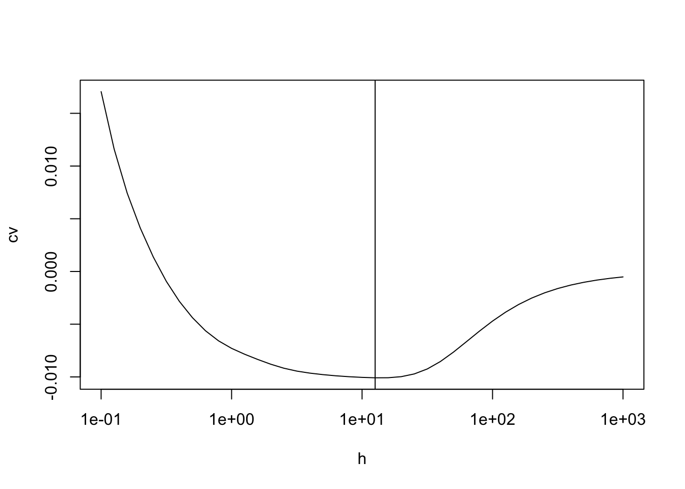
The optimal bandwidth is \(h = 12.59\). The kernel density estimate using this \(h\) is shown in the following figure.
x.min <- min(x) - 3*best.h
x.max <- max(x) + 3*best.h
m <- 100
x.tilde <- seq(x.min, x.max, length.out = m)

K <- dnorm(outer(x, x.tilde, "-"), sd = best.h)
f.hat <- colMeans(K)

plot(x.tilde, f.hat, type = "l",
     xlab = "snowfall [in]", ylab = "density")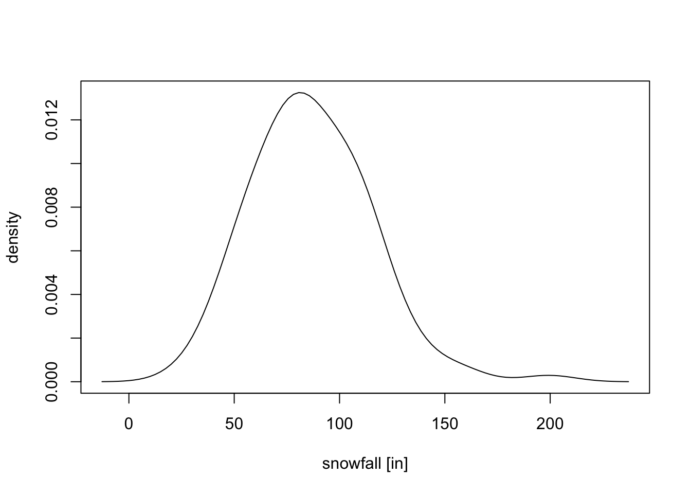
9.2 Kernel Regression
To illustrate cross-validation for the different smoothing methods,
we use the faithful dataset again.
We compare the methods using the leave-one-out mean squared error \[\begin{equation*} r(h) = \frac1n \sum_{i=1}^n \bigl( y_i - \hat m^{(i)}(x_i) \bigr)^2. \end{equation*}\]
We start by considering the Nadaraya-Watson estimator. Here we have to compute \[\begin{equation*} \hat m^{(i)}_h(x_i) = \frac{\sum_{j=1, j\neq i}^n K_h(x_i - x_j) y_j}{\sum_{j=1, j\neq i}^n K_h(x_i - x_j)} \end{equation*}\] for all \(i\in\{1, \ldots, n\}\). To evaluate this expression in R, we use the same ideas as before:
- We use
outer(x, x, "-")to compute all pair differences \(x_i - x_j\). - We use
dnorm(..., sd = h)to compute \(K_h\). - We can obtain the leave-one-out estimate by setting the diagonal of \(K\) to zero.
One new idea is needed to compute the products \(K_h(x_i - x_j) y_j\) in an efficient way:
- If we “multiply” a matrix
Kto a vectoryusing*(instead of using%*%for the usual matrix vector multiplication), the product is performed element-wise. Ifyhas as many elements asKhas rows, then the result is the matrix \((k_{ij}y_i)_{i,j}\), i.e. each row ofKis multiplied with the corresponding element ofy.
Combining these ideas, we get the following function to compute the leave-one-out estimate for the mean squared error of the Nadaraya-Watson estimator:
r.NW <- function(h) {
    K <- dnorm(outer(x, x, "-"), sd = h)

    # compute a leave-one-out estimate
    diag(K) <- 0

    m.hat <- colSums(K*y) / colSums(K)
    mean((m.hat - y)^2)
}
We will also consider local linear smoothing, i.e. local polynomial
smoothing where the degree \(p\) of the polynomials is \(p=1\).
As we have seen in the section about Polynomial Regression with Weights,
the local linear estimator can be computed as
\[\begin{equation*}
\hat m_h(x)
= e_0^\top (X^\top W X)^{-1} X^\top W y,
\end{equation*}\]
where \(X\) and \(W\) are defined as in equations (5.2)
and (5.1).
Here we use the “linear” case, \(p=1\).
For this case it is easy to check that we have
\[\begin{equation*}
X^\top W X
= \begin{pmatrix}
\sum_j K_h(x-x_j) & \sum_j K_h(x-x_j) x_j \\
\sum_j K_h(x-x_j) x_j & \sum_j K_h(x-x_j) x_j^2
\end{pmatrix}
\end{equation*}\]
and
\[\begin{equation*}
X^\top W y
= \begin{pmatrix}
\sum_j K_h(x-x_j) y_j \\
\sum_j K_h(x-x_j) x_j y_j
\end{pmatrix}.
\end{equation*}\]
Using the formula
\[\begin{equation*}
\begin{pmatrix}
a & b \\
c & d
\end{pmatrix}^{-1}
= \frac{1}{ad-bc} \begin{pmatrix}
d & -b \\
-c & a
\end{pmatrix}
\end{equation*}\]
for the inverse of a general \(2\times 2\)-matrix, we find
\[\begin{equation*}
\hat m_h(x)
= \frac{T_1 T_2 - T_3 T_4}{B_1 B_2 - B_3^2},
\end{equation*}\]
where
\[\begin{align*}
T_1 &= \sum_{j=1}^n K_h(x-x_j) y_j , \\
T_2 &= \sum_{j=1}^n K_h(x-x_j) x_j(x_j-x), \\
T_3 &= \sum_{j=1}^n K_h(x-x_j) x_j y_j , \\
T_4 &= \sum_{j=1}^n K_h(x-x_j) (x_j-x) , \\
B_1 &= \sum_{j=1}^n K_h(x-x_j) , \\
B_2 &= \sum_{j=1}^n K_h(x-x_j) x_j^2 , \\
B_3 &= \sum_{j=1}^n K_h(x-x_j) x_j .
\end{align*}\]
As before, for a leave-one-out estimate we need to compute these sums over all
\(j\neq i\). Since each of the seven terms listed above contains the term
\(K_h(x-x_j)\) inside the sum, we can achieve this by setting the corresponding
elements of the matrix K to zero.
r.LL <- function(h) {
    dx <- outer(x, x, "-")
    K <- dnorm(dx, sd = h)

    # compute a leave-one-out estimate
    diag(K) <- 0

    T1 <- colSums(y*K)
    T2 <- colSums(x*dx*K)
    T3 <- colSums(x*y*K)
    T4 <- colSums(dx*K)
    B1 <- colSums(K)
    B2 <- colSums(x^2*K)
    B3 <- colSums(x*K)
    m.hat <- (T1*T2 - T3*T4) / (B1*B2 - B3^2)

    mean((m.hat - y)^2)
}
Now we evaluate the function r.NW() and r.LL() on a grid of \(h\)-values
to find the optimal \(h\) for each method.
h <- 10^seq(-1.4, 0.1, length.out = 61)
mse.nw <- numeric(length(h))
mse.ll <- numeric(length(h))
for (i in seq_along(h)) {
    mse.nw[i] <- r.NW(h[i])
    mse.ll[i] <- r.LL(h[i])
}
plot(h, mse.nw, log="x", type = "l", ylim = range(mse.nw, mse.ll),
     ylab = "leave-one-out MSE")
lines(h, mse.ll, col="red")

best.h.NW <- h[which.min(mse.nw)]
abline(v = best.h.NW)
best.h.LL <- h[which.min(mse.ll)]
abline(v = best.h.LL, col="red")

legend("topleft", legend = c("NW", "LL"), col = c("black", "red"),
       lwd = 2)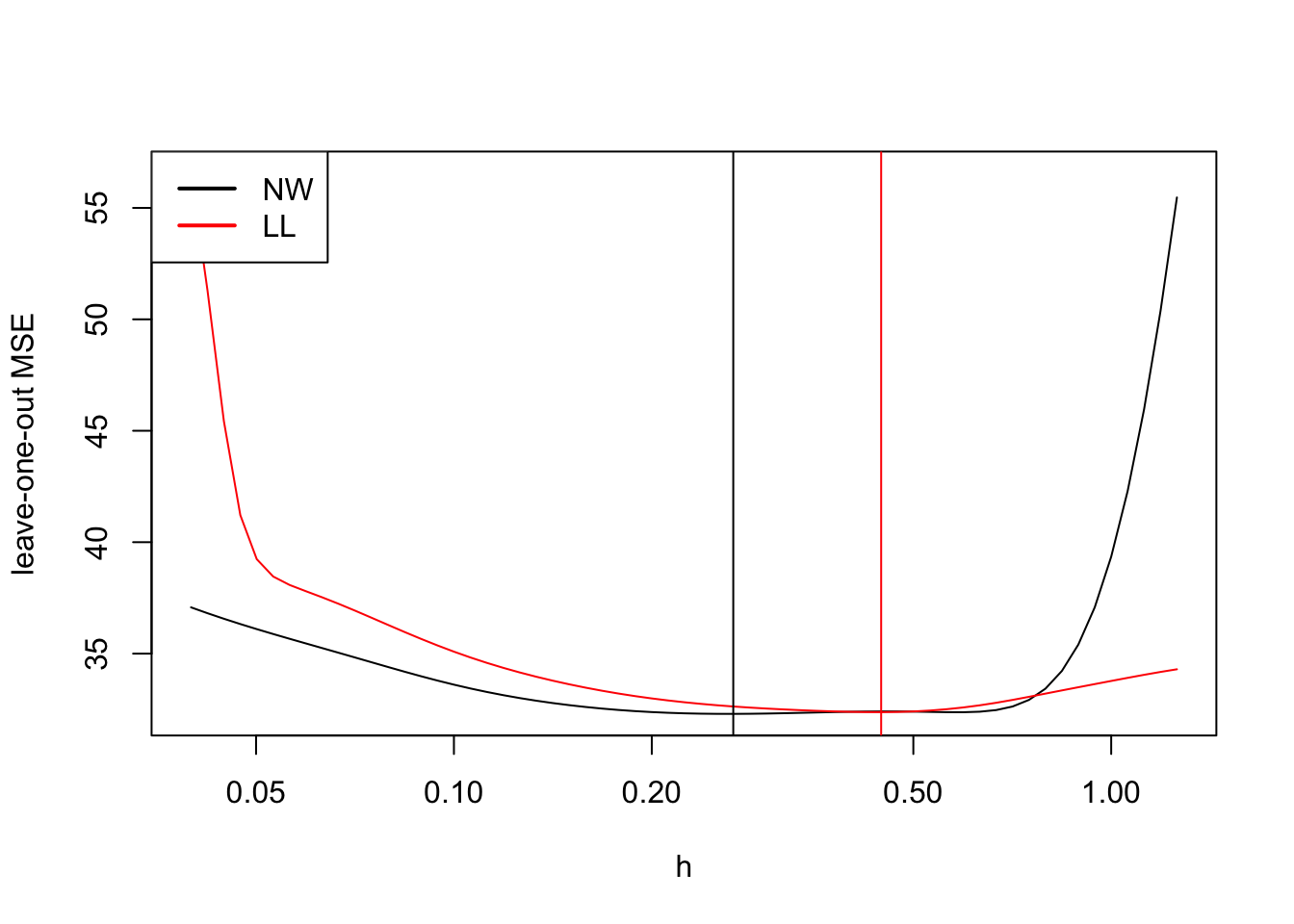
As expected, the optimal bandwidth for local linear regression is larger than for the Nadaraya-Watson estimator.
9.3 k-Nearest Neighbour Regression
To conclude this section we use leave-one-out cross-validation to determine the optimal \(k\) for \(k\)-nearest neighbour regression. Unlike KDE and kernel regression, where clever use of matrix operations allowed us to compute all leave-one-out predictions efficiently, kNN offers no such shortcut: removing observation \(i\) can change which points are the \(k\) nearest neighbours for every other observation. We therefore resort to a nested loop over both \(k\) values and observations, fitting a separate model for each combination. For this reason, the code in this section is much slower to run than the code in the previous sections.
k <- 10:70
mse.knn <- numeric(length(k))
for (j in seq_along(k)) {
    y.pred <- numeric(length(x))
    for (i in seq_along(x)) {
        m <- knn.reg(data.frame(x = x[-i]),
                     y = y[-i],
                     test = data.frame(x = x[i]),
                     k = k[j])
        y.pred[i] <- m$pred
    }
    mse.knn[j] <- mean((y - y.pred)^2)
}
plot(k, mse.knn, type = "l",
     ylab = "leave-one-out MSE")
best.k <- k[which.min(mse.knn)]
abline(v = best.k)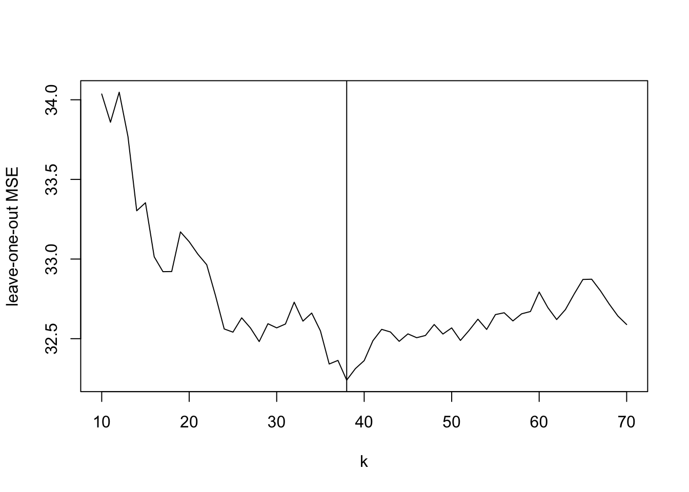
We note that the leave-one-out mean squared error for kNN is smaller than it is for Nadaraya-Watson or local linear regression, in the case of this dataset. Given the structure of the data, with different regions having very different densities of \(x\)-values, it makes sense that a method which chooses the bandwidth “adaptively” performs better.
To conclude, we show the optimal regression curves for the three smoothing methods together in one plot.
x.tilde <- seq(1.5, 5.5, length.out = 501)

K <- dnorm(outer(x, x.tilde, "-"), sd = best.h.NW)
m.NW <- colSums(K*y) / colSums(K)

dx <- outer(x, x.tilde, "-")
K <- dnorm(dx, sd = best.h.LL)
T1 <- colSums(y*K)
T2 <- colSums(x*dx*K)
T3 <- colSums(x*y*K)
T4 <- colSums(dx*K)
B1 <- colSums(K)
B2 <- colSums(x^2*K)
B3 <- colSums(x*K)
m.LL <- (T1*T2 - T3*T4) / (B1*B2 - B3^2)

m <- knn.reg(data.frame(x),
             y = y,
             test = data.frame(x=x.tilde),
             k = best.k)
m.kNN <- m$pred

colours <- c("#2C9CDA", "#811631", "#E0CA1D")
plot(x, y, xlim = range(x.tilde), cex = .5,
     xlab = "eruption time [mins]",
     ylab = "time to next eruption [mins]")
lines(x.tilde, m.NW, col = colours[1])
lines(x.tilde, m.LL, col = colours[2])
lines(x.tilde, m.kNN, col = colours[3])
legend("topleft", legend = c("NW", "LL", "kNN"), col = colours,
       lwd = 2)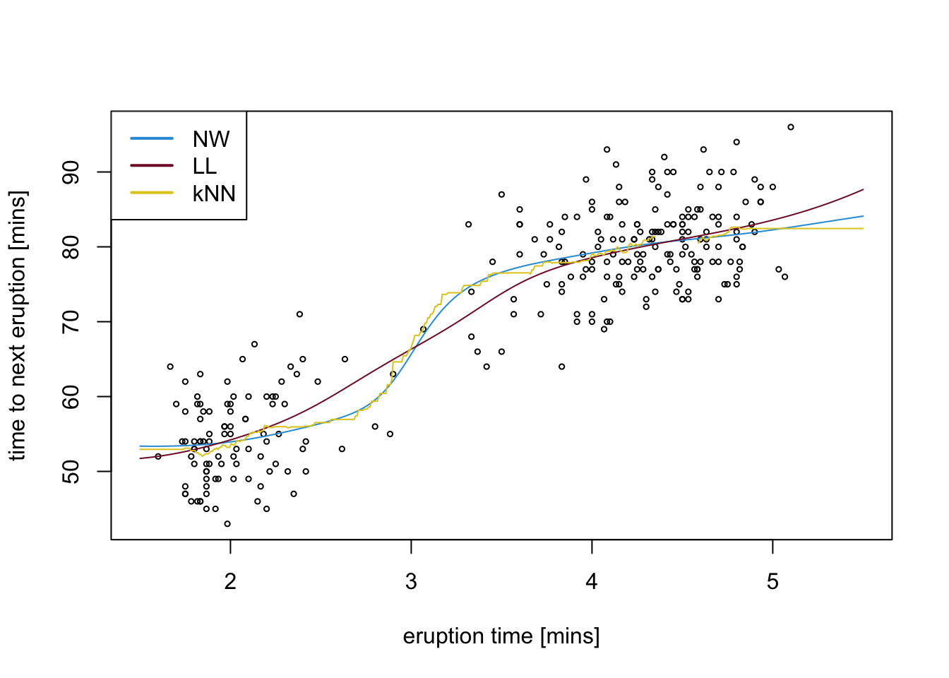
Summary
- Cross-validation for kernel density estimation uses integrated squared error or maximum likelihood criteria to select bandwidth \(h\).
- For kernel regression, leave-one-out cross-validation minimises \(\sum_i (y_i - \hat m_h^{(i)}(x_i))^2\) where \(\hat m_h^{(i)}\) excludes observation \(i\).
- Efficient implementation uses matrix operations with
outer()to compute all pairwise differences and kernel weights simultaneously. - The
faithfuldataset example shows that \(k\)-NN regression can outperform fixed-bandwidth methods when data density varies across the domain. - Optimal parameters differ between methods: local linear regression typically requires larger bandwidth than Nadaraya-Watson due to reduced boundary bias.