Section 1 Kernel Density Estimation

In this section we discuss the topic of “Kernel Density Estimation”. Here we suppose we are given data $x_1,\ldots, x_n \in\mathbb{R}^d$ from an unknown probability density, say $f$. Our objective is to estimate the density $f$. This section lays the foundations for many of the following topics.

1.1 Histograms

1.1.1 Probability Densities

Before we consider how to estimate a density, let us just remember what a density is. A random variable $X \in \mathbb{R}$ has density $f\colon \mathbb{R}\to [0, \infty)$ if \[\begin{equation*} P\bigl(X \in [a,b]\bigr) = \int_a^b f(x) \,dx \end{equation*}\] for all $a, b\in\mathbb{R}$ with $a < b$. Densities are sometimes also called “probability densities” or even “probability density functions”.

A density $f$ is large in regions where $X$ is very likely to take values, and small in regions where $X$ is less likely to take values. If $f(x) = 0$ for all $x$ in a region, that means that $X$ never takes values there. Graphically, the integral $\int_a^b f(x) \,dx$ can be interpreted as the area under the graph of $f$. This is illustrated in figure 1.1.

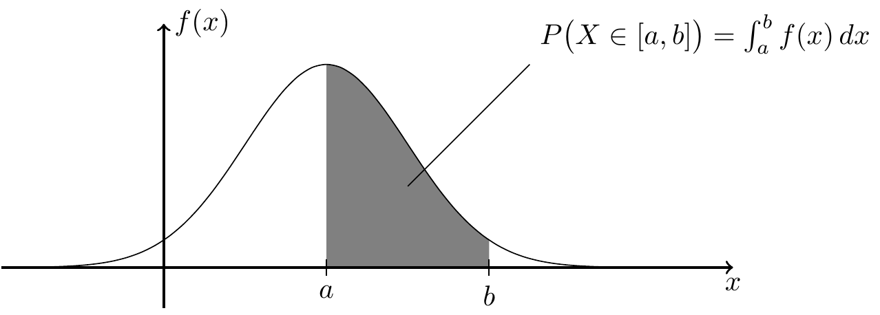
Figure 1.1: An illustration of how the area under the graph of a density can be interpreted as a probability.

A function $f$ is the density of some random variable $X$, if and only if $f \geq 0$ and \[\begin{equation*} \int_{-\infty}^\infty f(x) \,dx = 1. \end{equation*}\]

1.1.2 Histograms

In the univariate case, i.e. for $d = 1$, a commonly used technique to approximate the density of a sample is to plot a histogram. To illustrate this, we use the faithful dataset built in R, which contains waiting times between eruptions and the duration of the eruption for the Old Faithful geyser in the Yellowstone National Park. (You can type help(faithful) in R to learn more about this data set.) Here we focus on the waiting times only. A simple histogram for this dataset is shown in figure 1.2.

x <- faithful$waiting
hist(x, probability = TRUE,
     main = NULL, xlab = "time between eruptions [mins]")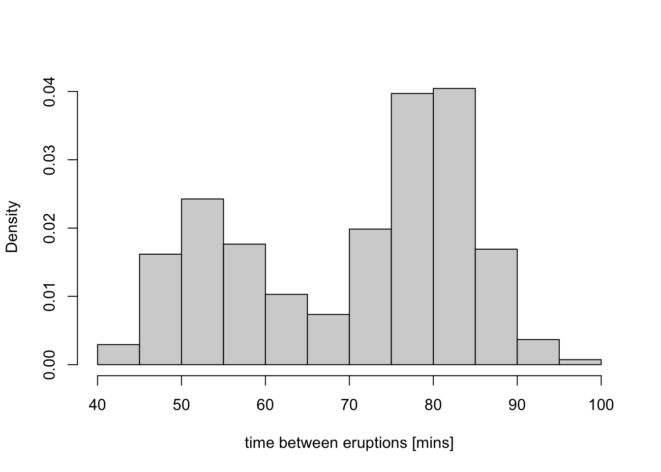

This figure shows how a histogram can be used to approximate a probability density. From the plot one can see that the density of the waiting times distribution seems to be bi-modal with peaks around 53 and 80 minutes.

Figure 1.2: This figure shows how a histogram can be used to approximate a probability density. From the plot one can see that the density of the waiting times distribution seems to be bi-modal with peaks around 53 and 80 minutes.

The histograms splits the range of the data into “buckets”, and for every bucket $[a, b]$ it shows a bar where the height is proportional the number of samples in the bucket. I am ignoring the case that a sample may fall exactly on the boundary between two buckets here; in reality all but one buckets need to be half-open intervals, for example $[40, 45]$, $(45, 50]$, …, $(95, 100]$.

As we have seen, the area under the graph of the density $f$ over the interval $[a, b]$ corresponds to the probability $P\bigl(X \in [a,b]\bigr)$. For the histogram to approximate the density, we need to scale the height $h_{a,b}$ of the bucket $[a, b]$ so that the area in the histogram is also close to this probability. Since we don’t know the probability $P\bigl(X \in [a,b]\bigr)$ exactly, we have to approximate it as \[\begin{equation*} P\bigl(X \in [a,b]\bigr) \approx \frac{n_{a,b}}{n}, \end{equation*}\] where $n_{a,b}$ is the number of samples in the bucket $[a,b]$, and $n$ is the total number of samples. So we need \[\begin{align*} (b-a) \cdot h_{a,b} &= \mbox{area of the histogram bar} \\ &\approx \mbox{area of the density} \\ &= P\bigl(X \in [a,b]\bigr) \\ &\approx \frac{n_{a,b}}{n}. \end{align*}\] and thus we choose \[\begin{equation*} h_{a,b} = \frac{1}{(b - a) n} n_{a,b}. \end{equation*}\] As expected, the height of the bar for the bucket $[a,b]$ is proportional to the number $n_{a,b}$ of samples in the bucket.

1.1.3 Choice of Buckets

Histograms are only meaningful if the buckets are chosen well. If the buckets are too large, not much of the structure of $f$ can be resolved. If the buckets are too small, the estimate $P\bigl(X \in [a,b]\bigr) \approx n_{a,b}/n$ will be poor and the histogram will no longer resemble the shape of $f$. This is for example demonstrated in figure 1.3.

set.seed(1)
x <- rnorm(50)
hist(x, probability = TRUE, main = NULL,
     breaks = seq(-2.5, 2.5, length.out = 500))

Figure 1.3: This figure demonstrates the consequences of choosing a too small bucket size.

Finally, even if reasonable bucket sizes are chosen, the result can depend quite strongly on the exact locations of these buckets. To illustrate this effect, we consider a dataset about the annual amount of snow falling in Buffalo, New York for different years. Figures 1.4 and 1.5 show the same data in two different ways, allowing to come to different conclusions about the distribution.

# downloaded from https://www1.maths.leeds.ac.uk/~voss/data/buffalo/
x <- read.csv("data/buffalo.csv")
snowfall <- x$snowfall
hist(snowfall, probability = TRUE,
     breaks = seq(24.30, 208.22, length.out = 20),
     main = NULL, xlab = "snowfall [in]")

The annual amount of snowfall in Buffalo, New York, in inches. The histogram makes it plausible that there is one main peak in the distribution.

Figure 1.4: The annual amount of snowfall in Buffalo, New York, in inches. The histogram makes it plausible that there is one main peak in the distribution.

hist(snowfall, probability = TRUE,
     breaks = seq(22.85, 204.92, length.out = 20),
     main = NULL, xlab = "snowfall [in]")

Figure 1.5: Continued from 1.4, this histogram shows the dataset in a way that three peaks are visible.

As a further illustration of the effect of bucket width, the code in figure 1.6 shows how histograms with different bucket widths can be generated in R. Here we simply specify numeric values for the break argument to hist(), which R uses as the approximate number of buckets in the plot.

par(mfrow = c(2,2))

for (breaks in c(80, 40, 20, 10)) {
  hist(snowfall,
       prob = TRUE,
       breaks = breaks,
       xlim = c(25,200),
       ylim = c(0, 0.03),
       xlab = paste("breaks =", breaks),
       main = NULL)
}

Figure 1.6: This figure illustrates how the bucket size in a histogram can be controlled in R.

1.2 Kernel Density Estimation

Kernel density estimation allows to estimate the density $f$ for given data while avoiding some of the disadvantages of histograms. Again, we suppose that we are given data $x_1, \ldots, x_n \in \mathbb{R}$ and that we want to estimate the density $f$.

1.2.1 Motivation

Similar to the argument in the previous subsection, for $x$ in a “small” interval $[a,b]$ we can estimate $f(x)$ as \[\begin{equation*} f(x) \approx \frac{1}{b-a} \int_a^b f(y) \,dy = \frac{1}{b-a} P\bigl( X\in [a,b] \bigr) \approx \frac{1}{b-a} \frac{n_{a,b}}{n}, \end{equation*}\] where $n_{a,b}$ denotes the number of samples in the interval $[a, b]$. This equation contains two approximation. The first one, $f(x) \approx 1/(ba) \int_a^b f(y) \,dy$, is more accurate if the interval is small, because then $f$ will be nearly constant over the interval. The second approximation will be more accurate if the interval is large, because then the interval $[a,b]$ covers more samples and the estimate of the probability is based on more data. We will later discuss in detail how these two concerns can be optimally balanced.

A mathematical “trick” to write more clearly how $n_{a,b}$ depends on the data is to write the value as \[\begin{equation*} n_{a,b} = \sum_{i=1}^n I_{[a,b]}(x_i), \end{equation*}\] where \[\begin{equation*} I_{[a,b]}(x) = \begin{cases} 1 & \mbox{if $x \in [a,b]$, and} \\ 0 & \mbox{otherwise.} \end{cases} \end{equation*}\] The function $I_{[a,b]}$ is called the indicator function of the set $[a, b]$.

Using the indicator function notation, the estimate for $f(x)$ can be written as \[\begin{align*} f(x) \approx \frac{1}{n(b-a)} n_{a,b} = \frac{1}{n} \sum_{i=1}^n \frac{1}{b-a} I_{[a,b]}(x_i) \end{align*}\] whenever $x \in [a,b]$ and when $b-a$ is “not too large and not too small”. For symmetry we choose the interval $[a, b]$ centred around $x$, say $[a, b] = [x - h, x + h]$ where $h$ can be chosen to control the width of the interval. In this case we have $b - a = x + h - x + h = 2h$ and thus \[\begin{align*} f(x) &\approx \frac{1}{n} \sum_{i=1}^n \frac{1}{2h} I_{[x-h,x+h]}(x_i) \\ &= \frac{1}{n} \sum_{i=1}^n \frac{1}{2h} I_{[-h,+h]}(x_i-x) \\ &= \frac{1}{n} \sum_{i=1}^n \frac{1}{2h} I_{[-1,+1]}\Bigl(\frac{x_i-x}{h}\Bigr) \end{align*}\] for all $x \in \mathbb{R}$. This is an example of a kernel density estimate. The function $K(x) = 1/2 \, I_{[-1,+1]}(x)$ on the right-hand side is called the kernel of the estimate, and the parameter $h$ is called the bandwidth or the smoothing parameter.

1.2.2 Definition of a Kernel Density Estimator

The general kernel density estimate is a generalisation of the idea from the previous subsection. We first define the class of functions which we use to replace the function $1/2 \, I_{[-1,+1]}$.

Definition 1.1 A kernel is a function $K\colon \mathbb{R}\to \mathbb{R}$ such that

$\int_{-\infty}^\infty K(x) \,dx = 1$,
$K(x) = K(-x)$ (i.e. $K$ is symmetric) and
$K(x) \geq 0$ (i.e. $K$ is positive) for all $x\in \mathbb{R}$.

Of these three properties, the first one is the most important one. The second condition, symmetry, ensures that $K$ is centred around $0$ and the third definition, positivity, makes $K$ a probability density. (While most authors list all three properties shown above, sometimes the third condition is omitted.)

It is easy to check that $K(x) = 1/2 \, I_{[-1,+1]}(x)$ satisfies all three conditions of definition 1.1. This function $K$ is sometimes called the “uniform kernel”, because it is the density of the uniform distribution $\mathcal{U}[-1,+1]$.

Based on the concept of a kernel, we now can define what a Kernel Density Estimate is.

Definition 1.2 For a kernel $K$, bandwidth $h > 0$ and $x \in \mathbb{R}$, the kernel density estimate for $f(x)$ is given by \[\begin{equation*} \hat f_h(x) = \frac{1}{n} \sum_{i=1}^n K_h(x - x_i), \end{equation*}\] where $K_h$ is given by \[\begin{equation*} K_h(y) = \frac{1}{h} K(y/h) \end{equation*}\] for all $y\in \mathbb{R}$.

For $K(x) = 1/2 \, I_{[-1,+1]}(x)$ this definition recovers the approximation we discussed in the previous section. In later sections we will see how the kernel $K$ can be chosen for the estimator $\hat f$ to have “good” properties. As a simple example we note that if $K$ is continuous, then the rescaled kernel $K_h$ and thus also the estimate $f_h$ are continuous functions.

Similar to the bucket width in histograms, the bandwidth parameter $h$ controls how smooth the density estimate $\hat f_h$ is, as a function of $x$.

1.2.3 Kernels

There are many different kernels in use. Some examples are listed below. A more exhautive list can, for example, be found on Wikipedia.

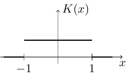
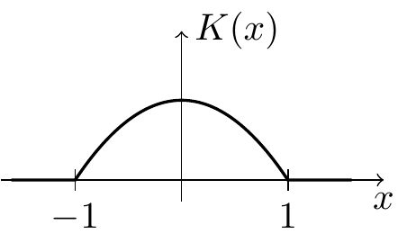
1.2.3.1 Uniform Kernel

\[\begin{equation*} K(x) = \begin{cases} 1/2 & \mbox{if $-1 \leq x \leq 1$} \\ 0 & \mbox{otherwise} \end{cases} \end{equation*}\]

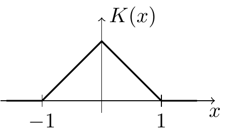
1.2.3.2 Triangular Kernel

\[\begin{equation*} K(x) = \begin{cases} 1-|x| & \mbox{if $-1 \leq x \leq 1$} \\ 0 & \mbox{otherwise} \end{cases} \end{equation*}\]

1.2.3.3 Epanechnikov Kernel

\[\begin{equation*} K(x) = \begin{cases} \frac34 (1-x^2) & \mbox{if $-1 \leq x \leq 1$} \\ 0 & \mbox{otherwise} \end{cases} \end{equation*}\]

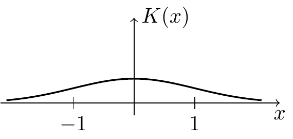
1.2.3.4 Gaussian Kernel

\[\begin{equation*} K(x) = \frac{1}{\sqrt{2\pi}} \exp\bigl(-x^2/2\bigr) \end{equation*}\]

1.3 Kernel Density Estimation in R

Kernel density estimates can be computed in R using the built-in density() function. If x is a vector containing the data, then density(x) computes a basic kernel density estimate, using the Gaussian kernel. The function has a number of optional arguments, which can be used to control details of the estimate:

bw = ... can be used to control the bandwidth $h$. If no numeric value is given, a heuristic is used. Note that for some kernels, bw differs from our $h$ by a constant factor. The value bw=1 always corresponds to the case where the probability distribution with density $K_h$ has variance 1.
kernel = ... can be used to choose the kernel. Choices incluse "rectangular" (the uniform kernel), "triangular", "epanechnikov" and "gaussian". The default value is "gaussian".

Details about how to call density() can be found by using the command help(density) in R.

The return value of density is an R object which contains information about the kernel density estimate.

m <- density(snowfall)
str(m)

## List of 7
##  $ x        : num [1:512] -4.17 -3.72 -3.26 -2.81 -2.35 ...
##  $ y        : num [1:512] 4.32e-06 4.98e-06 5.73e-06 6.56e-06 7.48e-06 ...
##  $ bw       : num 9.72
##  $ n        : int 109
##  $ call     : language density.default(x = snowfall)
##  $ data.name: chr "snowfall"
##  $ has.na   : logi FALSE
##  - attr(*, "class")= chr "density"

The fields $x and $y contain the $x$ and $y$ coordinates, respectively, of points on the $x \mapsto \hat f_h(x)$ curve, which approximates $f$. The field $bw shows the numeric value for the bandwidth chosen by the heuristic. The returned object can also directly be used as an argument to plot() and lines(), to add the graph of $\hat f_h$ to a plot.

The following code illustrates the use density() with different bandwidth bandwidth parameter. The result is shown in figure 1.7.

par(mfrow = c(2,2))

for (bw in c(1, 2, 4, 8)) {
  plot(density(snowfall, bw = bw, kernel = "triangular", n = 1000),
    xlim = c(25,200),
    ylim = c(0, 0.025),
    xlab = paste("bandwidth =", bw),
    main = NA)
}

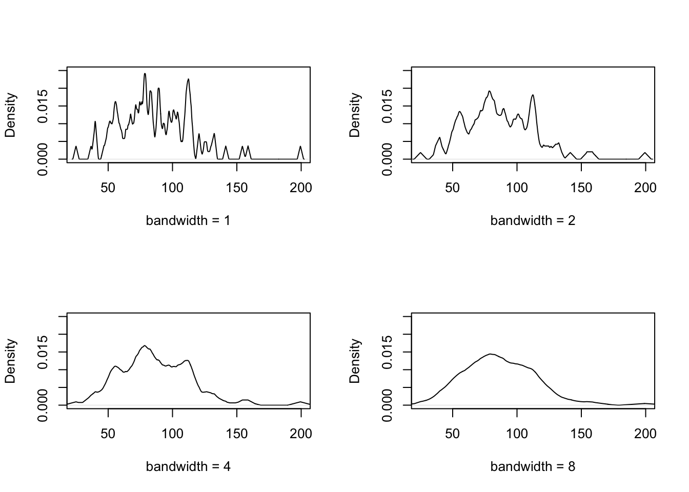
Figure 1.7: This figure illustrates how the bandwidth of a kernel density estimate can be controlled in R.

Summary

Histograms can be scaled so that they approximate densities.
Some care is needed when choosing buckets for a histogram.
Kernel density estimates can be used to estimate densities from data.
A variety of different kernel functions are commonly used.