Interlude: Kernel Density Estimation in R
In the previous section we have already seen how the function density()
can be used compute kernel density estimates in R. In the current section
we will compare different methods to compute these estimates “by hand”.
For out experiments we will use the same “snowfall” dataset as in the previous section.
# downloaded from https://teaching.seehuhn.de/data/buffalo/
x <- read.csv("data/buffalo.csv")
snowfall <- x$snowfall
Direct Implementation
The kernel density estimate for given data \(x_1, \ldots, x_n \in\mathbb{R}\) is \[\begin{equation*} \hat f_h(x) = \frac{1}{n} \sum_{i=1}^n K_h(x - x_i) = \frac{1}{n} \sum_{i=1}^n \frac{1}{h} K\Bigl( \frac{x - x_i}{h} \Bigr). \end{equation*}\] Our aim is to implement this formula in R.
To compute the estimate we need to choose a kernel function. For our experiment we use the triangular kernel from section 1.2.3.2:
The use of pmax() here allows to evaluate our newly defined function K()
for several \(x\)-values in parallel:
## [1] 0.0 0.5 1.0 0.5 0.0With this in place, we can now easily compute the kernel density estimate.
The triangular kernel used by the function density is scaled by a factor
\(1/\sqrt{6}\) compared to our formula, so here we use \(h = 4\sqrt{6}\)
to get output comparable to the density output for bw=4 (bottom left
panel in figure 1.7).
h <- 4 * sqrt(6) # bandwidth
x <- 100 # the point at which to estimate f
mean(1/h * K((x - snowfall) / h))
## [1] 0.0108237Typically we want to evaluate this function on a grid of \(x\)-values, for example to plot the estimated density \(\hat f\) as a function. Since \(x_1, \ldots, x_n\) is used to denote the input data, we need choose a different name for the \(x\)-values where we evaluate \(\hat f_h\). Here we use the \(\tilde x_1, \ldots \tilde x_m\) to denote these points:
x.tilde <- seq(25, 200, by = 1)
f.hat <- numeric(length(x.tilde)) # empty vector to store the results
for (j in 1:length(x.tilde)) {
  f.hat[j] <- mean(1/h * K((x.tilde[j] - snowfall) / h))
}
Plotting f.hat as a function x.tilde (figure 1.8) shows that we get a similar result
as we did in figure 1.7.
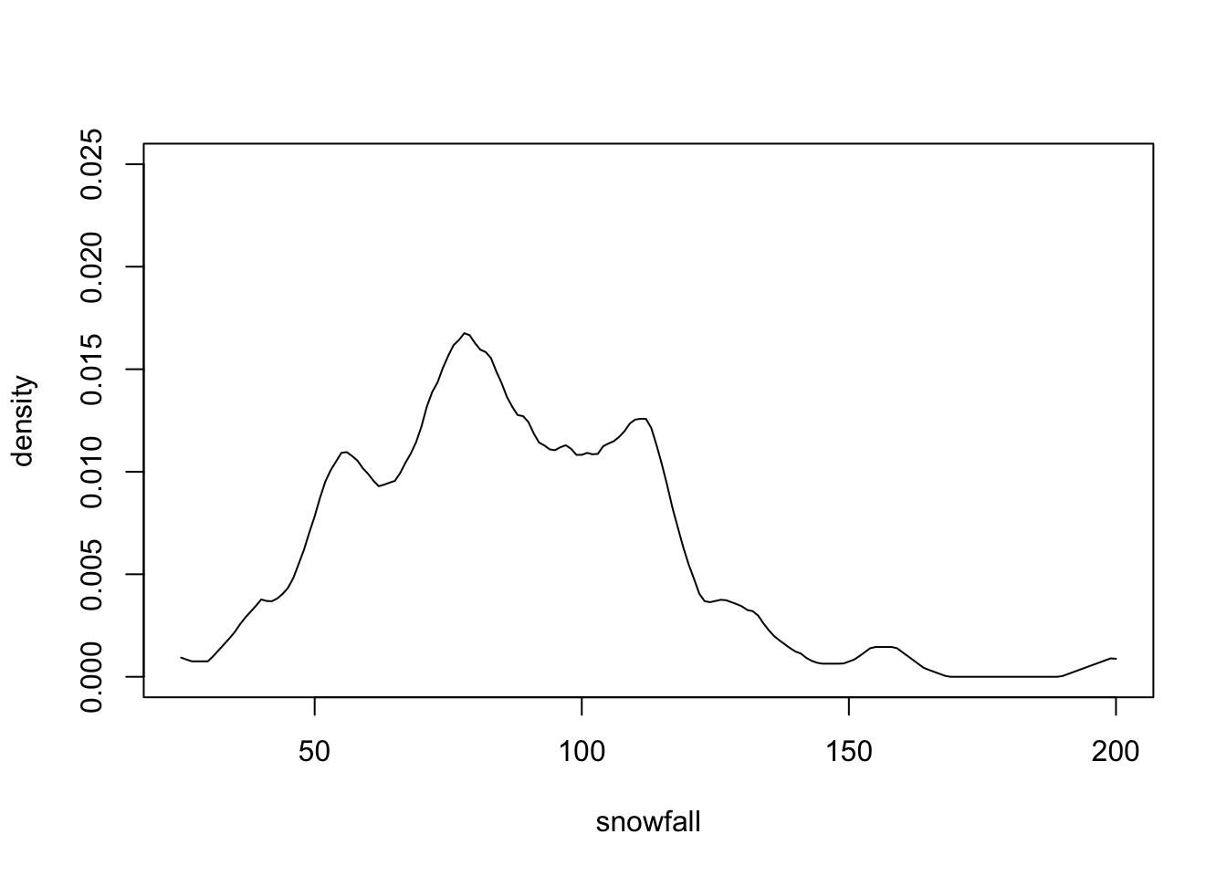
Figure 1.8: Manually computed kernel density estimate for the snowfall data, corresponding to bw=4 in density().
We will see in the next section that the code shown above is slower than
the built-in function density(), but on the other hand using our own code
we can control all details of the computation and there is no uncertainty
about what exactly the code does.
Speed Improvements
In this sub-section we will see how we can speed up our implementation of the kernel density estimate. To allow for easier speed comparisons, we encapsulate the code from above into a function:
KDE1 <- function(x.tilde, x, K, h) {
  f.hat <- numeric(length(x.tilde))
  for (j in 1:length(x.tilde)) {
    f.hat[j] <- mean(1/h * K((x.tilde[j] - x) / h))
  }
  f.hat
}
A common source of inefficiency in R code is the use of loops, like
the for-loop in the function KDE1(). The loop in our code
is used to compute the differences \(\tilde x_j - x_i\) for all \(j\).
We have already avoided a second loop by using the fact that
R interprets x.tilde[j] - x a vector operation, by using pmax()
in our implementation of K, and by using mean() to evaluate
the sum in the formula for \(\hat f_h\).
To also avoid the loop over j we can use the function outer(). This
function takes two vectors as inputs and then applies a function to all pairs
of elements from the two vectors. The result is a matrix where the rows
correspond to the elements of the first vector and the columns to the elements
of the second vector. The function to apply can either be an arithmetic
operation like "+" or "*", or an R-function which takes two numbers as
arguments. For example, the following code computes all pairwise differences
between the elements of two vectors:
##      [,1] [,2]
## [1,]    0   -1
## [2,]    1    0
## [3,]    2    1
Details about how to call outer() can be found by using the
command help(outer) in R.
We can use outer(x.tilde, x, "-") to compute all the \(\tilde x_j - x_i\)
at once. The result is a matrix with \(m\) rows and \(n\) columns, and
our implementation of the function K() can be applied to this matrix
to compute the kernel values for all values at once:
We will see at the end of this section that the function KDE2() is
significantly faster than KDE1(), and we can easily check that both
functions return the same result:
## [1] 0.0078239091 0.0108236983 0.0007448277## [1] 0.0078239091 0.0108236983 0.0007448277There is a another, minor optimisation we can make. Instead of dividing the
\(m\times n\) matrix elements of dx by h, we can achieve the same effect by
dividing the vectors x and x.tilde, i.e. only \(m+n\) numbers, by \(h\).
This reduces the number of operations required. Similarly, instead of
multiplying the \(m\times n\) kernel values by \(1/h\), we can divide the \(m\) row
means by \(h\):
Again, the new function KDE3() returns the same result as the original
implementation:
## [1] 0.0078239091 0.0108236983 0.0007448277To verify that our modifications really made the code faster, we measure
the execution times using the R package microbenchmark:
library("microbenchmark")

microbenchmark(
  KDE1 = KDE1(x.tilde, snowfall, K, h),
  KDE2 = KDE2(x.tilde, snowfall, K, h),
  KDE3 = KDE3(x.tilde, snowfall, K, h),
  times = 1000)
## Unit: microseconds
## expr min lq mean median uq max neval
## KDE1 1412.778 1476.9020 1566.8028 1496.9510 1521.0795 6546.880 1000
## KDE2 198.932 261.5390 333.3281 272.1375 281.9365 6038.070 1000
## KDE3 179.703 225.6025 301.7422 233.5360 241.7770 8802.618 1000The output summarises the execution times for 1000 runs of each of the
three functions. The columns correspond to the fastest measured time,
lower quartile, mean, median, upper quartile and slowest time, respectively.
(Different runs take different times, due to the fact that the computer
is busy with other tasks in the background.) We can see that the introduction
of outer() in KDE2() made a big difference, and that the further
optimisation in KDE3() improved speed further.
Finally, we compare the speed of our implementation to the built-in
function density(). To get comparable output we use the arguments
from, to, and n to specify the same grid \(\tilde x\)
as we used above.
KDE.builtin <- function(x.tilde, x, K, h) {
    density(x,
      kernel = K, bw = h / sqrt(6),
      from = min(x.tilde), to = max(x.tilde), n = length(x.tilde))$y
}
microbenchmark(density = KDE.builtin(x.tilde, snowfall, "triangular", h), times = 1000)
## Unit: microseconds
## expr min lq mean median uq max neval
## density 160.31 170.9905 189.1218 173.7375 177.5095 4533.534 1000The result shows that density() is faster than KDE3(), but by
a factor of less than 2. The reason is that density() uses a
more efficient algorithm for computing an approximation to
the kernel density estimate, based on Fast Fourier Transform.
By comparing the output of KDE.builtin() we can see that the
approximation used by density() gives nearly the same result as our
exact implementation of the method:
f.hat1 <- KDE3(x.tilde, snowfall, K, h)
f.hat2 <- KDE.builtin(x.tilde, snowfall, "triangular", h)
max(abs(f.hat1 - f.hat2))
## [1] 1.935582e-05