Interlude: Vectorisation in R
In this section we explore techniques for writing efficient R code, using kernel density estimation as an example. We start with a straightforward implementation using for-loops, then show how to speed it up by replacing loops with operations on entire vectors and matrices at once. These techniques apply to many computational problems in statistics.
For our experiments we will use the same “snowfall” dataset as in the previous section.
# downloaded from https://teaching.seehuhn.de/data/buffalo/
x <- read.csv("data/buffalo.csv")
snowfall <- x$snowfall
Direct Implementation
The kernel density estimate for given data \(x_1, \ldots, x_n \in\mathbb{R}\) is \[\begin{equation*} \hat f_h(x) = \frac{1}{n} \sum_{i=1}^n K_h(x - x_i) = \frac{1}{n} \sum_{i=1}^n \frac{1}{h} K\Bigl( \frac{x - x_i}{h} \Bigr). \end{equation*}\] Our aim is to implement this formula in R.
We use the triangular kernel from equation (1.2):
The use of pmax() allows us to evaluate K() for several \(x\)-values in parallel:
## [1] 0.0 0.5 1.0 0.5 0.0With this in place, we can now easily compute the kernel density estimate.
As mentioned in the previous section, the choice of kernel normalization and
bandwidth is not unique: rescaling the kernel and adjusting the bandwidth can
give the same \(K_h\). The R function density() uses a specific convention:
the bw parameter is defined to be the standard deviation of the smoothing kernel.
For the triangular kernel, this means that density() uses a rescaled version
with variance 1, which differs from our kernel in equation (1.2)
by a factor of \(1/\sqrt{6}\). Thus, to get output comparable to bw=4
(bottom left panel in figure 1.3), we use \(h = 4\sqrt{6}\):
h <- 4 * sqrt(6) # bandwidth
x <- 100 # the point at which to estimate f
mean(1/h * K((x - snowfall) / h))
## [1] 0.0108237To plot the estimated density, we typically evaluate \(\hat f_h\) on a grid of \(x\)-values. Since \(x_1, \ldots, x_n\) denotes the input data, we use \(\tilde x_1, \ldots, \tilde x_m\) for the evaluation points:
x.tilde <- seq(25, 200, by = 1)
f.hat <- numeric(length(x.tilde)) # empty vector to store the results
for (j in 1:length(x.tilde)) {
  f.hat[j] <- mean(1/h * K((x.tilde[j] - snowfall) / h))
}
Figure 1.4 shows the result is similar to figure 1.3.
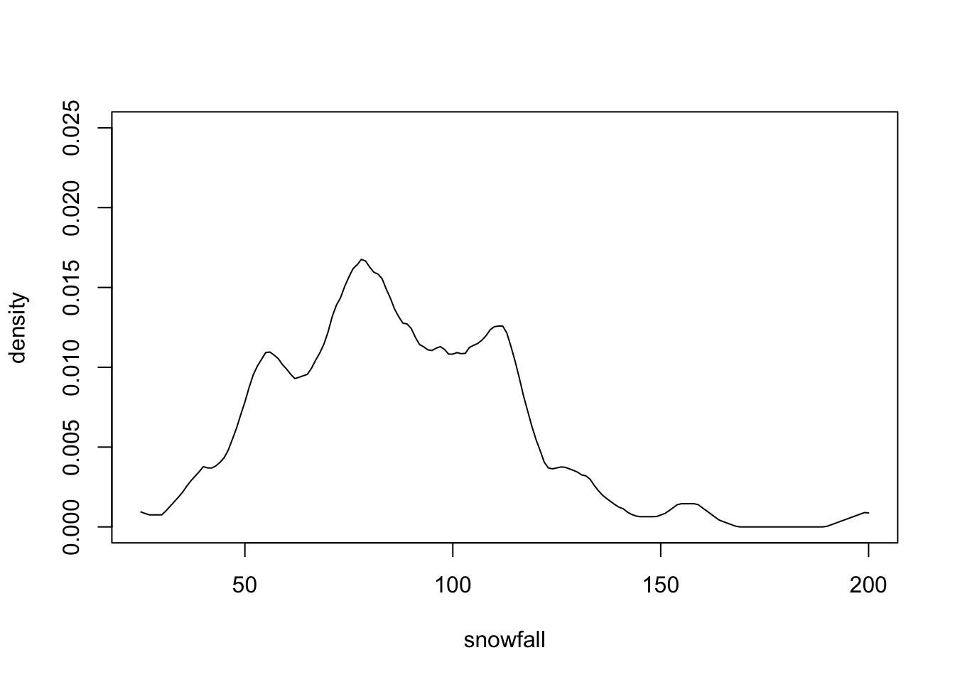
Figure 1.4: Manually computed kernel density estimate for the snowfall data, corresponding to bw=4 in density().
This code is slower than density() (as we will see below), but gives us full
control over the computation.
Vectorization
We now explore how to speed up our implementation. First, we encapsulate the code above into a function:
KDE1 <- function(x.tilde, x, K, h) {
  f.hat <- numeric(length(x.tilde))
  for (j in 1:length(x.tilde)) {
    f.hat[j] <- mean(1/h * K((x.tilde[j] - x) / h))
  }
  f.hat
}
A common source of inefficiency in R is the use of loops.
The for-loop in KDE1() computes differences \(\tilde x_j - x_i\) for all \(j\).
We have already avoided a second loop by treating x.tilde[j] - x as a vector
operation, using pmax() in K, and using mean() for the sum. This approach
of replacing explicit loops with operations on entire vectors is called vectorisation.
To eliminate the loop over j, we use outer(), which applies a function to all
pairs of elements from two vectors. The result is a matrix with rows corresponding
to the first vector and columns to the second. For example:
##      [,1] [,2]
## [1,]    0   -1
## [2,]    1    0
## [3,]    2    1
We use outer(x.tilde, x, "-") to compute all \(\tilde x_j - x_i\) at once,
giving an \(m \times n\) matrix to which we apply K(). This fully vectorised
implementation avoids all explicit loops:
We can verify that both functions return the same result:
## [1] 0.0078239091 0.0108236983 0.0007448277## [1] 0.0078239091 0.0108236983 0.0007448277There is another, minor optimisation we can make. Instead of dividing the
\(m\times n\) matrix elements of dx by h, we can achieve the same effect by
dividing the vectors x and x.tilde, i.e. only \(m+n\) numbers, by \(h\).
This reduces the number of operations required. Similarly, instead of
multiplying the \(m\times n\) kernel values by \(1/h\), we can divide the \(m\) row
means by \(h\):
Again, KDE3() returns the same result:
## [1] 0.0078239091 0.0108236983 0.0007448277We measure execution times using microbenchmark:
library("microbenchmark")

microbenchmark(
  KDE1 = KDE1(x.tilde, snowfall, K, h),
  KDE2 = KDE2(x.tilde, snowfall, K, h),
  KDE3 = KDE3(x.tilde, snowfall, K, h),
  times = 1000)
## Unit: microseconds
## expr min lq mean median uq max neval
## KDE1 808.889 821.9065 880.9922 837.753 861.6970 3811.237 1000
## KDE2 109.429 110.9460 151.1884 112.627 117.1575 2699.727 1000
## KDE3 97.990 99.6300 123.3287 101.147 105.3085 2660.613 1000The output shows execution times for 1000 runs. The introduction
of outer() in KDE2() gives a substantial speedup, and KDE3() improves further.
Finally, we compare to density(), using arguments from, to, and n
to specify the same grid \(\tilde x\):
KDE.builtin <- function(x.tilde, x, kernel_name, h) {
    density(x,
      kernel = kernel_name, bw = h / sqrt(6),
      from = min(x.tilde), to = max(x.tilde), n = length(x.tilde))$y
}
microbenchmark(density = KDE.builtin(x.tilde, snowfall, "triangular", h), times = 1000)
## Unit: microseconds
## expr min lq mean median uq max neval
## density 88.478 90.569 107.4159 100.04 103.7915 4162.73 1000The result shows that density() is faster than KDE3(), but by a factor
of less than 2. The reason is that density() uses a more efficient
algorithm based on Fast Fourier Transform to compute an approximation to the
kernel density estimate. By comparing the outputs of KDE3() and KDE.builtin()
we can see that the approximation is very accurate:
f.hat1 <- KDE3(x.tilde, snowfall, K, h)
f.hat2 <- KDE.builtin(x.tilde, snowfall, "triangular", h)
max(abs(f.hat1 - f.hat2))
## [1] 1.935582e-05Summary
- Vectorisation is the technique of replacing explicit loops with operations on entire vectors.
- Vectorised code dramatically improves performance in R.
- The
outer()function enables fully vectorised implementations for pairwise operations. - Further speedups can be achieved by reducing the number of operations on large matrices.