Problem Sheet 2
This problem sheet covers material from Sections 4-7 of the course. You should attempt all these questions and write up your solutions in advance of the workshop in week 4. Your solutions are not assessed. Instead, the answers will be discussed in the workshop and will be made available online afterwards.
5. Assume that \(X \sim \mathcal{N}(0, 1)\), \(Y\sim \chi^2(2)\) and \(Z \sim \chi^2(3)\) are independent. What are the distributions of the following random variables?
\(X^2\),
\(X^2 + Y + Z\),
\(\displaystyle\frac{\sqrt{2}X}{\sqrt{Y}}\),
\(\displaystyle\frac{2X^2}{Y}\), and
\(1.5\, Y/Z\).
The distributions involved in this question are the normal distribution, the \(\chi^2\)-dis-tri-bu-tion, the \(t\)-distribution and the \(F\)-distribution. The general rules are: (1) the sum of squares of \(d\) independent, standard normally distributed random variables follows a \(\chi^2(d)\)-distribution. (2) If \(Z\sim\mathcal{N}(0,1)\) and \(V \sim \chi^2(d)\) are independent, then \(Z / \sqrt{V / d} \sim t(d)\), and finally (3) If \(V_1\sim \chi^2(d_1)\) and \(V_2\sim \chi^2(d_2)\) are independent, then \((V_1/d_1)/(V_2/d_2) \sim F(d_1, d_2)\). Using these rules:
\(X^2 \sim \chi^2(1)\),
\(X^2 + Y + Z \sim \chi^2(1+2+3) = \chi^2(6)\),
\(\displaystyle\frac{\sqrt{2}X}{\sqrt{Y}} = \frac{X}{\sqrt{Y/2}} \sim t(2)\),
\(\displaystyle\frac{2X^2}{Y} = \frac{X^2/1}{Y/2} \sim F(1,2)\),
\(\displaystyle 1.5\, Y/Z = \frac{Y/2}{Z/3} \sim F(2, 3)\).
6. Let \(\mathbf{1} = (1, 1, \ldots, 1) \in\mathbb{R}^n\) and let \(X \sim \mathcal{N}(\mu, \sigma^2 I)\) be a normally-distributed random vector, where \(I\) is the \(n\times n\) identity matrix. Define \(A = \frac1n \mathbf{1} \mathbf{1}^\top \in \mathbb{R}^{n\times n}\).
Show that \((AX)_i = \bar X\) for all \(i \in \{1, \ldots, n\}\), where \(\bar X = \frac1n \sum_{j=1}^n X_j\).
Show that \(A\) is symmetric.
Show that \(A\) is idempotent.
Use results from lectures to conclude that the random variables \(AX\) and \(X^\top (I-A)X\) are independent.
Using the previous parts of the question, show that \(\bar X\) and \(\frac{1}{n-1} \sum_{i=1}^n (X_i - \bar X)^2\) are independent.
The matrix \(A = (a_{ij})\) has entries \(a_{ij} = 1/n\) for all \(i, j \in \{1, \ldots, n\}\). Using this observation, the statements of the first few questions follow easily:
We have \[\begin{equation*} (Ax)_i = \sum_{j=1}^n a_{ij} x_j = \sum_{j=1}^n \frac1n x_j = \frac1n \sum_{j=1}^n x_j = \bar x \end{equation*}\] for all \(i \in \{1, \ldots, n\}\).
We have \[\begin{equation*} a_{ij} = \frac1n = a_{ji} \end{equation*}\] for all \(i, j \in \{1, \ldots, n\}\) and thus \(A\) is symmetric.
We have \(\mathbf{1}^\top \mathbf{1} = \sum_{i=1}^n 1 \cdot 1 = n\) and thus \[\begin{equation*} A^2 = \bigl( \frac1n \mathbf{1} \mathbf{1}^\top \bigr) \bigl( \frac1n \mathbf{1} \mathbf{1}^\top \bigr) = \frac{1}{n^2} \mathbf{1} \bigl(\mathbf{1}^\top\mathbf{1}\bigr) \mathbf{1}^\top = \frac1n \mathbf{1} \mathbf{1}^\top = A. \end{equation*}\] (Alternatively, we could use the fact that we know the entries of \(A\) and compute \(A^2\) explicitly.)
For the remaining statements we will use the fact that \(X\) is normally distributed. We will repeatedly use the result that if two random variables \(X\) and \(Y\) are independent, that then any function of \(X\) is independent of any function of \(Y\).
In lectures we learned that, if \(A\) is symmetric and idempotent and if \(\varepsilon\sim \mathcal{N}(0, I)\), then \(A\varepsilon\) and \((I-A)\varepsilon\) are independent. Applying this result with \(\varepsilon= (X - \mu \mathbf{1}) / \sigma\) we find that \(AX = \sigma A\varepsilon+ \mu A \mathbf{1}\) and \((I-A)X = \sigma (I-A)\varepsilon+ \mu (I-A)\mathbf{1}\) are independent, since they are functions of \(A\varepsilon\) and \((I-A)\varepsilon\).
Since \((I - A)^\top (I - A) = I^2 - I A - A I + A^2 = I - A - A + A = I - A\) we have \[\begin{equation*} X^\top (I-A)X = X^\top (I - A)^\top (I-A)X = \Bigl( (I-A)X \Bigr)^\top \Bigl( (I-A)X \Bigr). \end{equation*}\] Thus, \(X^\top (I-A)X\) is a function of \((I-A)X\) and as such is also independent of \(AX\).
We have seen \((AX)_i = \bar X\) and thus \(\bigl((I - A)X\bigr)_i = X_i - \bar X\). This gives \[\begin{align*} X^\top (I-A)X &= \Bigl( (I-A)X \Bigr)^\top \Bigl( (I-A)X \Bigr) \\ &= \sum_{i=1}^n \Bigl( (I-A)X \Bigr)_i^2 \\ &= \sum_{i=1}^n (X_i - \bar X)^2 \end{align*}\] Thus we can write the sample mean as \(\bar X = (AX)_i\), and the sample variance as \(\mathrm{s}_X^2 = \frac{1}{n-1} \sum_{i=1}^n (X_i - \bar X)^2 = X^\top (I-A)X / (n-1)\), and if \(X\) is normally distributed the two values \(\bar X\) and \(\mathrm{s}_X^2\) are independent.
7. Consider the following R commands:
Call:
lm(formula = stack.loss ~ ., data = stackloss)

Residuals:
    Min      1Q  Median      3Q     Max
-7.2377 -1.7117 -0.4551  2.3614  5.6978

Coefficients:
            Estimate Std. Error t value Pr(>|t|)
(Intercept) -39.9197    11.8960  -3.356  0.00375 **
Air.Flow      0.7156     0.1349   5.307  5.8e-05 ***
Water.Temp    1.2953     0.3680   3.520  0.00263 **
Acid.Conc.   -0.1521     0.1563  -0.973  0.34405
---
Signif. codes:  0 '***' 0.001 '**' 0.01 '*' 0.05 '.' 0.1 ' ' 1

Residual standard error: 3.243 on 17 degrees of freedom
Multiple R-squared:  0.9136,    Adjusted R-squared:  0.8983
F-statistic:  59.9 on 3 and 17 DF,  p-value: 3.016e-09
Either using this output, or using R to further inspect the built-in
stackloss dataset, find a \(99\%\)-confidence interval for the
parameter \(\beta_\mathtt{Acid.Conc.}\).
From lectures, we know that a confidence interval for a single coefficient \(\beta_j\) is given by \[\begin{equation*} [U, V] = \Bigl[ \hat\beta_j - t_{n-p-1}(\alpha/2) \sqrt{\widehat{\sigma^2} C_{jj}}, \hat\beta_j + t_{n-p-1}(\alpha/2) \sqrt{\widehat{\sigma^2} C_{jj}} \Bigr], \end{equation*}\] where \(t_{n-p-1}\) is the \((1-\alpha/2)\)-quantile of the \(t\)-distribution, \(C_{jj} = (X^\top X)^{-1}_{jj}\), and \(X\) is the design matrix.
We can read off the required values for computing the confidence
interval from the output of summary(m): the centre of the
confidence interval can be found in the column Estimate, the
standard error \(\sqrt{\widehat{\sigma^2} C_{jj}}\) is given in column
Std. Error, and the value \(n-p-1\) for the \(t\)-quantile can be
found as the degrees of freedom for the residual standard error,
near the bottom of the output. Using these values, we can find a
\(95\%\)-confidence interval for Acid.Conc. as
follows:
[1] -0.6050934 0.3008934Thus, the confidence interval is \(\bigl[ -0.605, 0.301 \bigr]\).
8. The file 20211020.csv from
contains pairs of \((x, y)\) values. Fit the following models to the data:
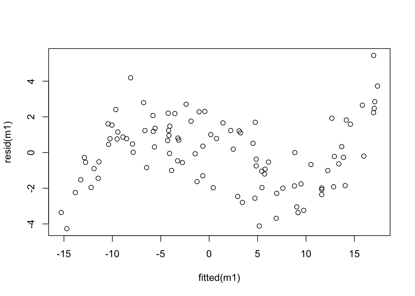
\(y = \beta_0 + \beta_1 x + \varepsilon\)
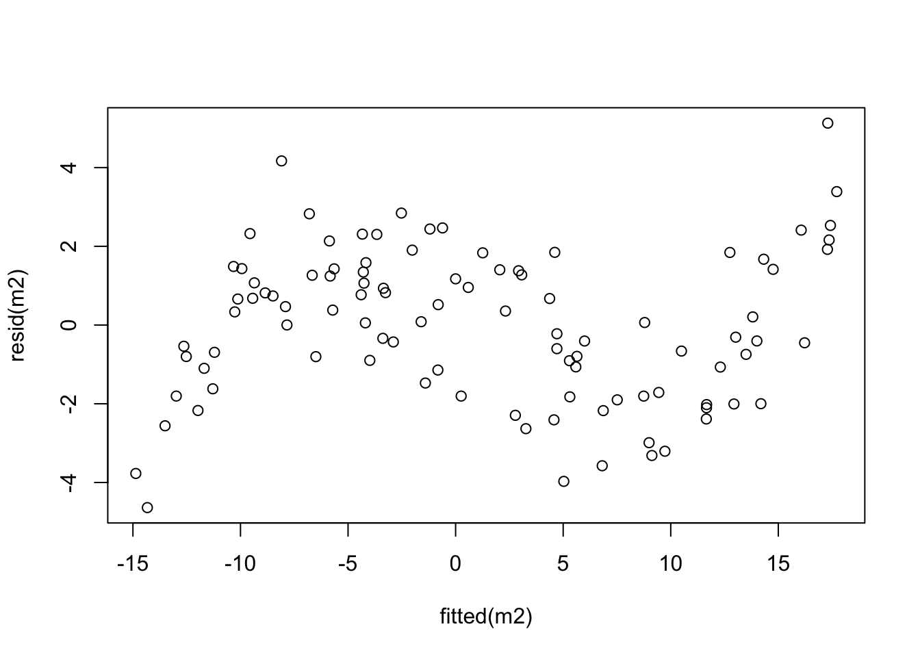
\(y = \beta_0 + \beta_1 x + \beta_2 x^2 + \varepsilon\)
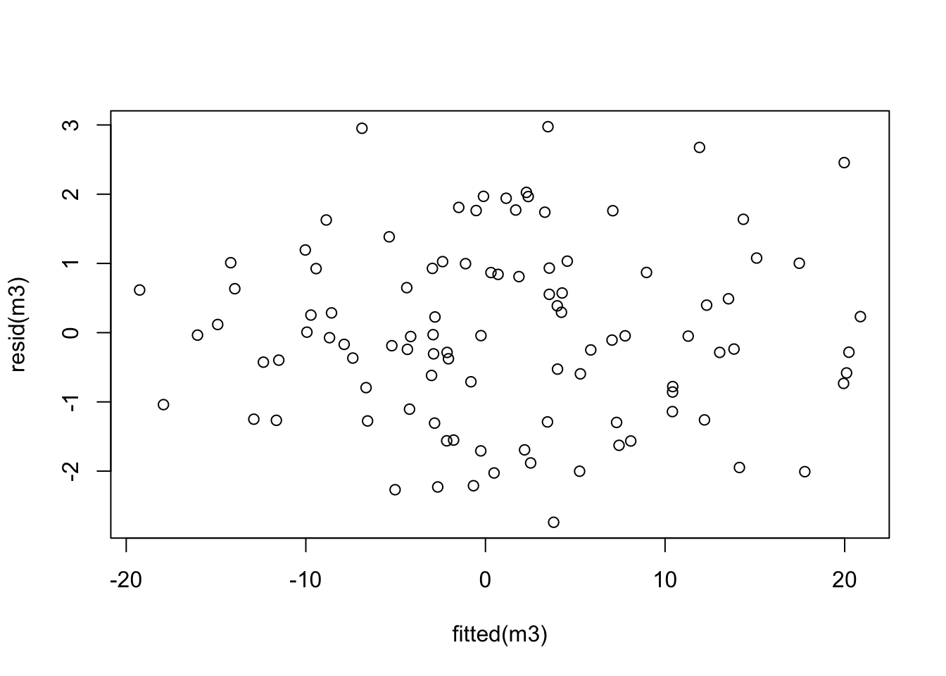
\(y = \beta_0 + \beta_1 x + \beta_2 x^2 + \beta_3 x^3 + \varepsilon\)
For each model, create a “residual plot”, i.e. a scatter plot which has the fitted values on the horizontal axis and the residuals on the vertical axis. Comment on the resulting plots.