MATH3714 Linear Regression and Robustness
University of Leeds, Semester 1, 2025/26
Preface
From previous modules we know how to fit a regression line through points \((x_1, y_1), \ldots, (x_n, y_n) \in\mathbb{R}^2\). The underlying model here is described by the equation \[\begin{equation*} y_i = \alpha + \beta x_i + \varepsilon_i \end{equation*}\] for all \(i \in \{1, 2, \ldots, n\}\), and the aim is to find values for the intercept \(\alpha\) and the slope \(\beta\) such that the fitted line is as close as possible to the data points. This procedure, called simple linear regression, is illustrated in figure 0.1. The variables \(x_i\) are called input, “features”, “predictors”, or sometimes also “explanatory variables” or “independent variables”. The variables \(y_i\) are called output or “response”, or sometimes the “dependent variables”. The values \(\varepsilon_i\) are called the errors or noise terms.
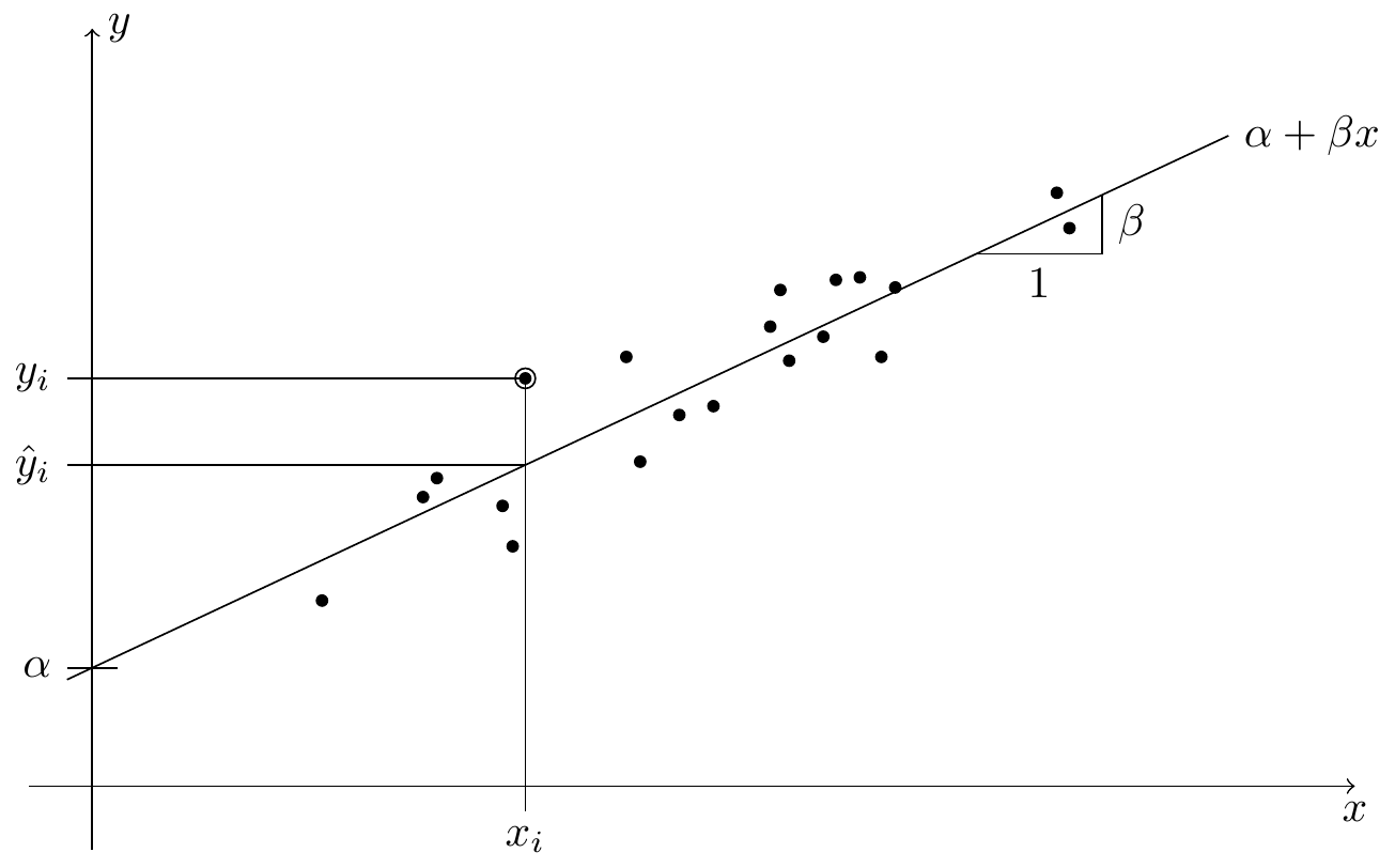
Figure 0.1: An illustration of linear regression. Each of the black circles in the plot stands for one paired sample \((x_i, y_i)\). The regression line \(x \mapsto \alpha + \beta x\), with intercept \(\alpha\) and slope \(\beta\), aims to predict the value of \(y\) using the observed value \(x\). For the marked sample \((x_i, y_i)\), the predicted \(y\)-value is \(\hat y_i\).
Extending the situation of simple linear regression, here we will consider multiple linear regression, where the response \(y\) is allowed to depend on several input variables. The corresponding model is now \[\begin{equation*} y_i = \beta_0 + \beta_1 x_{i1} + \cdots + \beta_p x_{ip} + \varepsilon_i \end{equation*}\] for all \(i \in \{1, 2, \ldots, n\}\), where \(n\) is still the number of observations, and \(p\) is now the number of inputs we observe for each sample. The aim is now to find values for the intercept \(\beta_0\) and the slopes \(\beta_1, \ldots, \beta_p\) such that the fitted hyperplane is as close as possible to the data points. Note that for multiple linear regression, we still consider a single response for each sample, only the number of inputs has been increased.
We will discuss multiple linear regression in much detail; our discussion will answer questions like the following:
- Given a new input \(x\), how can we predict the corresponding output \(y\)?
- By studying a fitted regression model, sometimes better understanding of the data can be achieved. For example, one could ask whether all of the \(p\) input variables carry information about the response \(y\). We will use statistical hypothesis tests to answer such questions.
- How well does the model fit the data?
- How to deal with outliers in the data?
In the next section, we will begin by reviewing simple linear regression in detail, before moving on to the multiple regression case.