Section 2 Least Squares Estimates
2.1 Data and Models
For multiple linear regression we assume that there are \(p\) inputs and one output. If we have a sample of \(n\) observations, we have \(np\) inputs and \(n\) outputs in total. Here we denote the \(i\)th observation of the \(j\)th input by \(x_{ij}\) and the corresponding output by \(y_i\).
As an example, we consider the mtcars dataset built into R. This is a small
dataset, which contains information about 32 automobiles (1973-74 models). The
table lists fuel consumption mpg, gross horsepower hp, and 9 other aspects
of these cars. Here we consider mpg to be the output, and the other listed
aspects to be inputs. Type help(mtcars) in R to learn more about this
dataset:
                     mpg cyl  disp  hp drat    wt  qsec vs am gear carb
Mazda RX4           21.0   6 160.0 110 3.90 2.620 16.46  0  1    4    4
Mazda RX4 Wag       21.0   6 160.0 110 3.90 2.875 17.02  0  1    4    4
Datsun 710          22.8   4 108.0  93 3.85 2.320 18.61  1  1    4    1
Hornet 4 Drive      21.4   6 258.0 110 3.08 3.215 19.44  1  0    3    1
Hornet Sportabout   18.7   8 360.0 175 3.15 3.440 17.02  0  0    3    2
Valiant             18.1   6 225.0 105 2.76 3.460 20.22  1  0    3    1
Duster 360          14.3   8 360.0 245 3.21 3.570 15.84  0  0    3    4
Merc 240D           24.4   4 146.7  62 3.69 3.190 20.00  1  0    4    2
Merc 230            22.8   4 140.8  95 3.92 3.150 22.90  1  0    4    2
Merc 280            19.2   6 167.6 123 3.92 3.440 18.30  1  0    4    4
Merc 280C           17.8   6 167.6 123 3.92 3.440 18.90  1  0    4    4
Merc 450SE          16.4   8 275.8 180 3.07 4.070 17.40  0  0    3    3
Merc 450SL          17.3   8 275.8 180 3.07 3.730 17.60  0  0    3    3
Merc 450SLC         15.2   8 275.8 180 3.07 3.780 18.00  0  0    3    3
Cadillac Fleetwood  10.4   8 472.0 205 2.93 5.250 17.98  0  0    3    4
Lincoln Continental 10.4   8 460.0 215 3.00 5.424 17.82  0  0    3    4
Chrysler Imperial   14.7   8 440.0 230 3.23 5.345 17.42  0  0    3    4
Fiat 128            32.4   4  78.7  66 4.08 2.200 19.47  1  1    4    1
Honda Civic         30.4   4  75.7  52 4.93 1.615 18.52  1  1    4    2
Toyota Corolla      33.9   4  71.1  65 4.22 1.835 19.90  1  1    4    1
Toyota Corona       21.5   4 120.1  97 3.70 2.465 20.01  1  0    3    1
Dodge Challenger    15.5   8 318.0 150 2.76 3.520 16.87  0  0    3    2
AMC Javelin         15.2   8 304.0 150 3.15 3.435 17.30  0  0    3    2
Camaro Z28          13.3   8 350.0 245 3.73 3.840 15.41  0  0    3    4
Pontiac Firebird    19.2   8 400.0 175 3.08 3.845 17.05  0  0    3    2
Fiat X1-9           27.3   4  79.0  66 4.08 1.935 18.90  1  1    4    1
Porsche 914-2       26.0   4 120.3  91 4.43 2.140 16.70  0  1    5    2
Lotus Europa        30.4   4  95.1 113 3.77 1.513 16.90  1  1    5    2
Ford Pantera L      15.8   8 351.0 264 4.22 3.170 14.50  0  1    5    4
Ferrari Dino        19.7   6 145.0 175 3.62 2.770 15.50  0  1    5    6
Maserati Bora       15.0   8 301.0 335 3.54 3.570 14.60  0  1    5    8
Volvo 142E          21.4   4 121.0 109 4.11 2.780 18.60  1  1    4    2
For this dataset we have \(n = 32\) (number of cars), and \(p = 10\) (number
of predictors, excluding mpg). The values \(y_1, \ldots, y_{32}\) are listed
in the first column of the table, the values \(x_{i,1}\) for \(i \in \{1, \ldots,
32\}\) are shown in the second column, and the values \(x_{i,10}\) are shown in
the last column.
It is easy to make scatter plots which show how a single input affects the output. For example, we can show how the engine power affects fuel consumption:
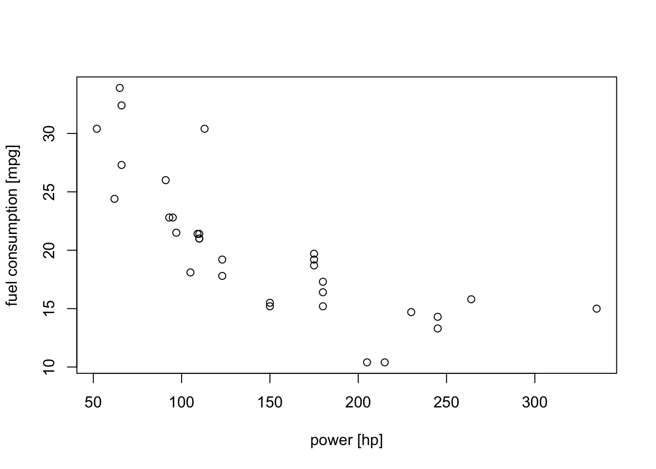
We can see that cars with stronger engines tend to use more fuel (i.e. a gallon of fuel lasts for fewer miles; the curve goes down), but leaving out the other inputs omits a lot of information. It is not easy to make a plot which takes all inputs into account. It is also not immediately obvious which of the variables are most important.
In linear regression, we assume that the output depends on the inputs in a linear way. We write this as \[\begin{equation} y_i = \beta_0 + \beta_1 x_{i,1} + \cdots + \beta_p x_{i,p} + \varepsilon_i \tag{2.1} \end{equation}\] where the errors \(\varepsilon_i\) are assumed to be “small”. Here, \(i\) ranges over all \(n\) samples, so (2.1) represents \(n\) simultaneous equations. The parameters \(\beta_j\) can be interpreted as the expected change in the response \(y\) per unit change in \(x_j\) when all other inputs are held fixed.
This model describes a hyperplane in the \((p+1)\)-dimensional space of the inputs \(x_j\) and the output \(y\). The hyperplane is easily visualized when \(p=1\) (as a line in \(\mathbb{R}^2\)), and visualisation can be attempted for \(p=2\) (as a plane in \(\mathbb{R}^3\)) but is hard for \(p>2\).
2.2 The Normal Equations
Similar to what we did in Section 1.3, we rewrite the model using matrix notation. We define the vectors \[\begin{equation*} y = \begin{pmatrix} y_1 \\ y_2 \\ \vdots \\ y_n \end{pmatrix} \in \mathbb{R}^n, \qquad \varepsilon= \begin{pmatrix} \varepsilon_1 \\ \varepsilon_2 \\ \vdots \\ \varepsilon_n \end{pmatrix} \in \mathbb{R}^n, \qquad \beta = \begin{pmatrix} \beta_0 \\ \beta_1 \\ \vdots \\ \beta_p \end{pmatrix} \in\mathbb{R}^{1+p} \end{equation*}\] as well as the matrix \[\begin{equation*} X = \begin{pmatrix} 1 & x_{1,1} & \cdots & x_{1,p} \\ 1 & x_{2,1} & \cdots & x_{2,p} \\ \vdots & \vdots & & \vdots \\ 1 & x_{n,1} & \cdots & x_{n,p} \\ \end{pmatrix} \in \mathbb{R}^{n\times (1+p)}. \end{equation*}\] The parameters \(\beta_i\) are called the regression coefficients and the matrix \(X\) is called the design matrix.
Using this notation, the model (2.1) can be written as \[\begin{equation} y = X \beta + \varepsilon, \tag{2.2} \end{equation}\] where again \(X\beta\) is a matrix-vector multiplication which “hides” the sums in equation (2.1), and (2.2) is an equation of vectors of size \(n\), which combines the \(n\) individual equations from (2.1).
To simplify notation, we index the columns of \(X\) by \(0, 1, \ldots, p\) (instead of the more conventional \(1, \ldots, p+1\)), so that we can for example write \[\begin{equation*} (X \beta)_i = \sum_{j=0}^p x_{i,j} \beta_j = \beta_0 + \sum_{j=1}^p x_{i,j} \beta_j. \end{equation*}\]
As before, we find the regression coefficients by minimising the residual sum of squares: \[\begin{align*} r(\beta) &= \sum_{i=1}^n \varepsilon_i^2 \\ &= \sum_{i=1}^n \bigl( y_i - (\beta_0 + \beta_1 x_{i,1} + \cdots + \beta_p x_{i,p}) \bigr)^2. \end{align*}\] In practice, this notation turns out to be cumbersome, and we will use matrix notation in the following proof.
Lemma 2.1 Assume that the matrix \(X^\top X \in \mathbb{R}^{(1+p) \times (1+p)}\) is invertible. Then the function \(r(\beta)\) takes its minimum at the vector \(\hat\beta\in\mathbb{R}^{p+1}\) given by \[\begin{equation*} \hat\beta = (X^\top X)^{-1} X^\top y. \end{equation*}\]
Proof. Using the vector equation \(\varepsilon= y - X \beta\), we can also write the residual sum of squares as \[\begin{align*} r(\beta) &= \sum_{i=1}^n \varepsilon_i^2 \\ &= \varepsilon^\top \varepsilon\\ &= (y - X \beta)^\top (y - X \beta) \\ &= y^\top y - y^\top X\beta - (X\beta)^\top y + (X\beta)^\top (X\beta). \end{align*}\] Using the linear algebra rules from Appendix A.2 we find that \(y^\top X\beta = (X\beta)^\top y = \beta^\top X^\top y\) and \((X\beta)^\top (X\beta) = \beta^\top X^\top X \beta\). Thus we get \[\begin{equation*} r(\beta) = y^\top y - 2\beta^\top X^\top y + \beta^\top X^\top X \beta. \end{equation*}\] Note that in this equation \(X\) is a matrix, \(y\) and \(\beta\) are vectors, and \(r(\beta)\) is a number.
To find the minimum of this function, we set all partial derivatives \(\frac{\partial}{\partial \beta_i} r(\beta)\) equal to \(0\). Going through the terms in the formula for \(r(\beta)\) we find: (1) \(y^\top y\) does not depend on \(\beta\), so we have \(\frac{\partial}{\partial \beta_i} y^\top y = 0\) for all \(i\), (2) we have \[\begin{equation*} \frac{\partial}{\partial \beta_i} \beta^\top X^\top y = \frac{\partial}{\partial \beta_i} \sum_{j=0}^p \beta_j (X^\top y)_j = (X^\top y)_i \end{equation*}\] and (3) finally \[\begin{equation*} \frac{\partial}{\partial \beta_i} \beta^\top X^\top X \beta = \frac{\partial}{\partial \beta_i} \sum_{j,k=0}^p \beta_j (X^\top X)_{j,k} \beta_k = 2 \sum_{k=0}^p (X^\top X)_{i,k} \beta_k = 2 \bigl( (X^\top X) \beta \bigr)_i. \end{equation*}\] (Some care is needed, when checking that the middle equality sign in the previous equation is correct.) Combining these derivatives, we find \[\begin{equation} \frac{\partial}{\partial \beta_i} r(\beta) = 0 - 2 (X^\top y)_i + 2 \bigl( X^\top X \beta \bigr)_i \tag{2.3} \end{equation}\] for all \(i \in \{0, 1, \ldots, p\}\). At a local minimum of \(r\), all of these partial derivatives must be zero and using a vector equation we find that a necessary condition for a minimum is \[\begin{equation} X^\top X \beta = X^\top y. \tag{2.4} \end{equation}\] Since we assumed that \(X^\top X\) is invertible, there is exactly one vector \(\beta\) which solves (2.4). This vector is given by \[\begin{equation*} \hat\beta := (X^\top X)^{-1} X^\top y. \end{equation*}\]
As for one-dimensional minimisation, there is a condition on the second derivatives which must be checked to see which local extrema are local minima. Here we are only going to sketch this argument: A sufficient condition for \(\hat\beta\) to be a minimum is for the second derivative matrix (the Hessian matrix) to be positive definite (see appendix A.2.8). Using equation (2.3) we find \[\begin{equation*} \frac{\partial^2}{\partial\beta_i \partial\beta_j} r(\beta) = 2 (X^\top X)_{i,j} \end{equation*}\] And thus the Hessian matrix is \(H = 2 X^\top X\). Using results from linear algebra, one can show that this matrix is indeed positive definite and thus \(\hat\beta\) is the unique minimum of \(r\).
Equation (2.4) gives a system of \(p+1\) linear equations with \(p+1\) unknowns. This system of linear equations, \(X^\top X \beta = X^\top y\) is called the normal equations. If \(X^\top X\) is invertible, as assumed in the lemma, this system of equations has \(\hat\beta\) as its unique solution. Otherwise, there may be more than one \(\beta\) which leads to the same value \(r(\beta)\) and the minimum will no longer be unique. This happens for example, if two of the inputs are identical to each other (or, more generally, one input is linearly dependent on one or more other inputs).
The condition that \(X^\top X\) must be invertible in lemma 2.1 corresponds to the condition \(\mathrm{s}_x^2 > 0\) in lemma 1.1.
The value \(\hat\beta\) found in the lemma is called the least squares estimator for \(\beta\).
2.3 Fitted Values
Let us again consider our model \[\begin{equation*} y = X \beta + \varepsilon, \end{equation*}\] using the matrix notation introduced above. Here we can think of \(X\beta\) as the true values, while \(\varepsilon\) are the errors. Using the least squares estimate \(\hat\beta\) we can estimate the true values as \[\begin{equation} \hat y = X \hat\beta. \tag{2.5} \end{equation}\] These estimates are called the fitted values. Using the definition of \(\hat\beta\) we get \[\begin{equation*} \hat y = X (X^\top X)^{-1} X^\top y =: Hy. \end{equation*}\] The matrix \(H = X (X^\top X)^{-1} X^\top\) is commonly called the hat matrix (because it “puts the hat on \(y\)”).
Finally, we can estimate the errors using the residuals \[\begin{equation} \hat\varepsilon = y - X \hat\beta = y - \hat y = y - H y = (I - H) y, \tag{2.6} \end{equation}\] where \(I\) is the \(n\times n\) identity matrix.
2.4 Example
To conclude this section, we demonstrate how these methods can be used
in R. For this we consider the mtcars example from the beginning of
the section again. We will first see how to do the analysis “by hand”,
and later show how the same result can be obtained using R’s built-in functions.
We first split mtcars into the response column y (the first column)
and the design matrix X (a column of ones, followed by columns 2 to 11
of mtcars):
Next we compute \(X^\top X\) and solve the normal equations. Often it is faster, easier, and has smaller numerical errors to solve the normal equations rather than inverting the matrix \(X^\top X\).
            [,1]
     12.30337416
cyl  -0.11144048
disp  0.01333524
hp   -0.02148212
drat  0.78711097
wt   -3.71530393
qsec  0.82104075
vs    0.31776281
am    2.52022689
gear  0.65541302
carb -0.19941925
Without further checks it is hard to know whether the result is correct, or
whether we made a mistake somewhere. One good sign is that we argued earlier
that higher hp should lead to lower mpg, and indeed the corresponding
coefficient -0.02148212 is negative.
Finally, compute the fitted values and generate a plot of fitted values against responses. If everything worked, we would expect the points in this plot to be close to the diagonal.
y.hat <- X %*% beta.hat
plot(y, y.hat, xlab = "responses", ylab = "fitted values")
abline(a = 0, b = 1) # plot the diagonal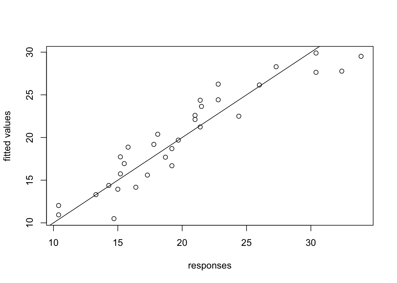
For comparison we now re-do the analysis using built-in R commands.
In the lm() command below, we use data=mtcars to tell R where the
data is stored, and the formula mpg ~ . states that we want to
model mpg as a function of all other variable (this is the meaning of .).
(Intercept)         cyl        disp          hp        drat          wt
12.30337416 -0.11144048  0.01333524 -0.02148212  0.78711097 -3.71530393
       qsec          vs          am        gear        carb
 0.82104075  0.31776281  2.52022689  0.65541302 -0.19941925
Comparing these coefficients to the vector beta.hat from above shows
that we got the same result using both methods. The fitted values
can be computed using fitted.values(m). Here we just check that we get
the same result as above:
[1] 3.979039e-13This result 3.410605e-13 stands for the number \(3.410605 \cdot 10^{-13}\),
which is extremely small. The difference between our results and R’s result
is caused by rounding errors.
2.5 Models Without Intercept
Sometimes, it is useful to fit a model without an intercept. This means that we assume that the output \(y\) is a linear function of the inputs \(x_1, \ldots, x_p\) but that the output is zero when all inputs are zero. We write this as \[\begin{equation*} y_i = \beta_1 x_{i,1} + \cdots + \beta_p x_{i,p} + \varepsilon_i \end{equation*}\] for all \(i \in \{1, \ldots, n\}\).
When we write this model in matrix notation, we need to leave out the intercept column in the design matrix \(X\). For this case we get \[\begin{equation*} y = \begin{pmatrix} y_1 \\ y_2 \\ \vdots \\ y_n \end{pmatrix} \in \mathbb{R}^n, \qquad \varepsilon= \begin{pmatrix} \varepsilon_1 \\ \varepsilon_2 \\ \vdots \\ \varepsilon_n \end{pmatrix} \in \mathbb{R}^n, \qquad \beta = \begin{pmatrix} \beta_1 \\ \vdots \\ \beta_p \end{pmatrix} \in\mathbb{R}^p \end{equation*}\] as well as the matrix \[\begin{equation*} X = \begin{pmatrix} x_{1,1} & \cdots & x_{1,p} \\ x_{2,1} & \cdots & x_{2,p} \\ \vdots & & \vdots \\ x_{n,1} & \cdots & x_{n,p} \\ \end{pmatrix} \in \mathbb{R}^{n\times p}. \end{equation*}\] The vectors \(y\) and \(\varepsilon\) are unchanged, but the vector \(\beta\) is now shorter and the matrix \(X\) is narrower.
Most of the results in this module carry over to this case, for example the least squares estimate for \(\beta\) is still given by \[\begin{equation*} \hat\beta = (X^\top X)^{-1} X^\top y. \end{equation*}\] However, some results need to be adjusted and to be sure one has to carefully check the details of the derivations when results are needed for models without intercept.
Summary
- Multiple linear regression allows for more than one input, but still has only one output.
- The least squared estimate for the coefficients is found by minimising the residual sum of squares.
- The least squares estimate can be computed by solving the normal equations.
- The hat matrix transforms responses into fitted values.
- Residuals estimate the errors as \(\hat\varepsilon= y - \hat y\).
- Models can be fitted without an intercept term when appropriate.