Section 16 Ridge Regression
In cases where \(X\) shows approximate multicollinearity, the parameter estimates \(\hat\beta\) have coefficients with large variance. In case of exact multicollinearity, \(\hat\beta\) is no longer uniquely defined, and the minimum of the residual sum of squares is attained on an unbounded subspace of the parameter space. In both cases, a more stable estimate can be obtained by changing the estimation procedure to include an additional penalty term which discourages “large” values of \(\hat\beta\). This is the idea of ridge regression. In this section we will see that the resulting estimates are biased, but sometimes have smaller mean squared error than the least squares estimator.
16.1 Definition of the Estimator
Definition 16.1 In multiple linear regression, the ridge regression estimate for the parameter vector \(\beta\) is given by \[\begin{equation} \hat\beta^{(\lambda)} = \mathop{\mathrm{arg\,min}}\limits_\beta \Bigl( \sum_{i=1}^n \bigl( y_i - (X \beta)_i \bigr)^2 + \lambda \|\beta\|^2 \Bigr). \end{equation}\] The parameter \(\lambda \geq 0\) is called the regularisation parameter.
Here we write \(\mathop{\mathrm{arg\,min}}\limits\nolimits_\beta (\cdots)\) to denote the value of \(\beta\) which minimises the expression on the right-hand side, and \(\|\beta\|\) denotes the Euclidean norm of the vector \(\beta\), i.e. \[\begin{equation*} \|\beta\|^2 = \sum_{j=0}^p \beta_j^2. \end{equation*}\]
The term being minimised is \[\begin{equation*} r^{(\lambda)}(\beta) = \sum_{i=1}^n \bigl( y_i - (X \beta)_i \bigr)^2 + \lambda \|\beta\|^2, \end{equation*}\] consisting of the residual sum of squares plus a penalty term. The regularisation parameter \(\lambda\) controls the relative weight of these two terms. For large \(\lambda\), the main objective is to minimise the norm \(\|\beta\|\) and one can show that \(\lim_{\lambda \to\infty} \hat\beta^{(\lambda)} = 0\). For \(\lambda \downarrow 0\) only the residual sum of squares is left and if \(X^\top X\) is invertible we get \(\hat\beta^{(0)} = \hat\beta\), i.e. here the ridge regression estimate coincides with the least squares estimate.
As in lemma 2.1 we can find an explicit formula for the ridge regression estimate. For this we write \(r^{(\lambda)}\) as \[\begin{equation*} r^{(\lambda)}(\beta) = (y - X\beta)^\top (y - X\beta) + \lambda \beta^\top \beta \end{equation*}\] and then take derivatives to find the minimum. The result is given by \[\begin{equation*} \hat\beta^{(\lambda)} = (X^\top X + \lambda I)^{-1} X^\top y. \end{equation*}\]
Example 16.1 To illustrate the method, we compute the ridge regression estimate for a badly conditioned toy dataset.
# fix the true parameters for our simulated data:
beta <- c(0, .5, .5)
sigma <- 0.01

set.seed(20211112)
x1 <- c(1.01, 2.00, 2.99, 4.02, 5.01, 5.99)
x2 <- c(0.98, 1.99, 3.00, 4.00, 4.99, 6.00)
# beta[1] in R corresponds to \beta_0, beta[2] = \beta_1, beta[3] = \beta_2
y <- beta[1] + beta[2] * x1 + beta[3] * x2 + rnorm(6, 0, sigma)

lambda <- 0.01
X <- model.matrix(y ~ x1 + x2)
beta.ridge <- solve(t(X) %*% X + lambda * diag(ncol(X)), t(X) %*% y)
beta.ridge[,1] # get first column instead of n × 1 matrix, for tidiness
(Intercept) x1 x2
-0.01620501 0.52739367 0.47343531 For comparison, we also compute the least squares estimate:
(Intercept)          x1          x2
-0.02935851  1.03064453 -0.02749857
We see that despite the small value of \(\lambda\) there is a considerable difference between the estimated values \(\hat\beta\) and \(\hat\beta^{(\lambda)}\) in this example. Experimenting with different values of the seed also shows that the variance of \(\hat\beta^{(\lambda)}\) is much smaller than the variance of \(\hat\beta\). Below we will see a theoretical explanation for this fact.
For \(\lambda > 0\) and \(v \neq 0\) we have \(\|v\| > 0\) and thus \[\begin{align*} \| (X^\top X + \lambda I) v \|^2 &= v^\top (X^\top X + \lambda I)^\top (X^\top X + \lambda I) v \\ &= v^\top X^\top X X^\top X v + 2 \lambda v^\top X^\top X v + \lambda^2 v^\top v \\ &= \| X X^\top X v \|^2 + 2 \lambda \| X v \|^2 + \lambda^2 \| v \|^2 \\ &\geq \lambda^2 \| v \|^2 \\ &> 0. \end{align*}\] This shows, by theorem A.1, that the matrix \(X^\top X + \lambda I\) is invertible for every \(\lambda > 0\). Thus the ridge regression estimate for \(\lambda > 0\) is always uniquely defined, even in cases where the least squares estimate is not uniquely defined.
There are variants of the method where the penalty term \(\|\beta\|^2\) is replaced with a different penalty term. One example of this is Lasso (least absolute shrinkage and selection operator) regression, which uses \(\|\beta\|_1 = \sum_{j=0}^p |\beta_j|\) as the penalty term.
Outside statistics, ridge regression is known as Tikhonov regularisation.
16.2 Properties of the Estimate
Using the statistical model \[\begin{equation*} Y = X \beta + \varepsilon \end{equation*}\] as before, we have \[\begin{align*} \hat\beta^{(\lambda)} &= (X^\top X + \lambda I)^{-1} X^\top Y \\ &= (X^\top X + \lambda I)^{-1} X^\top (X \beta + \varepsilon) \\ &= (X^\top X + \lambda I)^{-1} (X^\top X + \lambda I) \beta \\ &\hskip15mm - (X^\top X + \lambda I)^{-1} \lambda I \beta \\ &\hskip15mm + (X^\top X + \lambda I)^{-1} X^\top \varepsilon \end{align*}\] and simplifying the first term on the right-hand side we get \[\begin{equation} \hat\beta^{(\lambda)} = \beta - \lambda (X^\top X + \lambda I)^{-1} \beta + (X^\top X + \lambda I)^{-1} X^\top \varepsilon. \tag{16.1} \end{equation}\]
16.2.1 Bias
Using the formula for \(\hat\beta^{(\lambda)}\) we get \[\begin{equation*} \mathbb{E}\bigl( \hat\beta^{(\lambda)} \bigr) = \beta - \lambda (X^\top X + \lambda I)^{-1} \beta + 0 \end{equation*}\] and thus \[\begin{equation*} \mathop{\mathrm{bias}}\bigl( \hat\beta^{(\lambda)} \bigr) = - \lambda (X^\top X + \lambda I)^{-1} \beta. \end{equation*}\] Since this term in general is non-zero, we see that \(\hat\beta^{(\lambda)}\) is a biased estimate. The amount of bias depends on the unknown, true coefficient vector \(\beta\).
16.2.2 Variance
The covariance matrix of the vector \(\hat\beta^{(\lambda)}\) is given by \[\begin{align*} \mathop{\mathrm{Cov}}\bigl(\hat\beta^{(\lambda)}\bigr) &= \mathop{\mathrm{Cov}}\Bigl( \beta - \lambda (X^\top X + \lambda I)^{-1} \beta + (X^\top X + \lambda I)^{-1} X^\top \varepsilon \Bigr) \\ &= \mathop{\mathrm{Cov}}\Bigl( (X^\top X + \lambda I)^{-1} X^\top \varepsilon \Bigr) \\ &= (X^\top X + \lambda I)^{-1} X^\top \mathop{\mathrm{Cov}}(\varepsilon) X (X^\top X + \lambda I)^{-1} \\ &= \sigma^2 (X^\top X + \lambda I)^{-1} X^\top X (X^\top X + \lambda I)^{-1} \\ &= \sigma^2 (X^\top X + \lambda I)^{-1} - \lambda \sigma^2 (X^\top X + \lambda I)^{-2}. \end{align*}\] While this is an explicit formula, the resulting covariance matrix depends on the unknown error variance \(\sigma^2\).
If \(X^\top X\) is invertible, this covariance will converge to the covariance of the least squares estimator as \(\lambda \downarrow 0\). From this we can find the variance of individual components as \(\mathop{\mathrm{Var}}\bigl( \hat\beta^{(\lambda)}_j \bigr) = \mathop{\mathrm{Cov}}( \hat\beta^{(\lambda)} )_{jj}\).
16.2.3 Mean Squared Error
The Mean Squared Error (MSE) of an estimator \(\hat \beta_j\) for \(\beta_j\) is given by \[\begin{equation*} \mathop{\mathrm{MSE}}\nolimits( \hat\beta_j ) = \mathbb{E}\Bigl( \bigl( \hat\beta_j - \beta_j \bigr)^2 \Bigr). \end{equation*}\] It is an easy exercise to show that this can equivalently be written as \[\begin{equation*} \mathop{\mathrm{MSE}}\nolimits\bigl( \hat\beta_j \bigr) = \mathop{\mathrm{Var}}\bigl( \hat\beta_j \bigr) + \mathop{\mathrm{bias}}\bigl( \hat\beta_j \bigr)^2. \end{equation*}\] Using the formulas for the variance and bias from above, we can find a formula for \(\mathop{\mathrm{MSE}}\nolimits(\hat\beta^{(\lambda)}_j)\), but the result is hard to interpret. Instead of considering these analytical expressions, we illustrate the MSE using a numerical example.
Example 16.2 Continuing from example 16.1 above, we can determine the MSE for every value of \(\lambda\). Here we use the fact that this is simulated data where we know the true values of \(\beta\) and \(\sigma^2\).
We start with the bias:
lambda <- 0.1
Q <- t(X) %*% X + lambda * diag(ncol(X))
y <- X %*% beta
lambda * solve(Q, t(X) %*% y)
[,1]
(Intercept) 0.0009178679
x1 0.0497789499
x2 0.0499545553For the covariance matrix we get the following:
C1 <- solve(Q) # Compute the inverse Q^{-1} ...
C2 <- C1 %*% C1 # ... and also Q^{-2}, to get
sigma^2 * (C1 - lambda*C2) # the covariance matrix.
(Intercept) x1 x2
(Intercept) 7.291379e-05 -7.580602e-06 -9.226941e-06
x1 -7.580602e-06 3.831264e-06 -1.540098e-06
x2 -9.226941e-06 -1.540098e-06 4.221464e-06Now we repeat these calculations in a loop, to plot the MSE as a function of \(\lambda\):
lambda <- 10^seq(-4, 0, length.out = 100) # range of lambda to try
j.plus.1 <- 1 + 1 # we plot the error of \beta_1

variance <- numeric(length(lambda))
bias <- numeric(length(lambda))
for (i in seq_along(lambda)) {
    lambda.i <- lambda[i]
    Q <- t(X) %*% X + lambda.i * diag(ncol(X))
    C1 <- solve(Q)
    bias[i] <- (lambda.i * solve(Q, t(X) %*% X %*% beta))[j.plus.1]
    C2 <- C1 %*% C1
    C <- C1 - lambda.i*C2
    variance[i] <- sigma^2 * C[j.plus.1, j.plus.1]
}
MSE <- variance + bias^2

plot(lambda, MSE, type = "l", log = "x", ylim = c(0, 0.1))
lines(lambda, bias^2, col="#1b9e77", lwd = 3)
lines(lambda, variance, col="#d95f02", lwd = 3)
lines(lambda, MSE) # make sure MSE is not obscured by bias/variance
abline(v = lambda[which.min(MSE)]) # mark the minimum

legend("topleft",
       c("bias squared", "variance", "MSE"),
       col = c("#1b9e77", "#d95f02", "black"),
       lwd = c(3, 3, 1))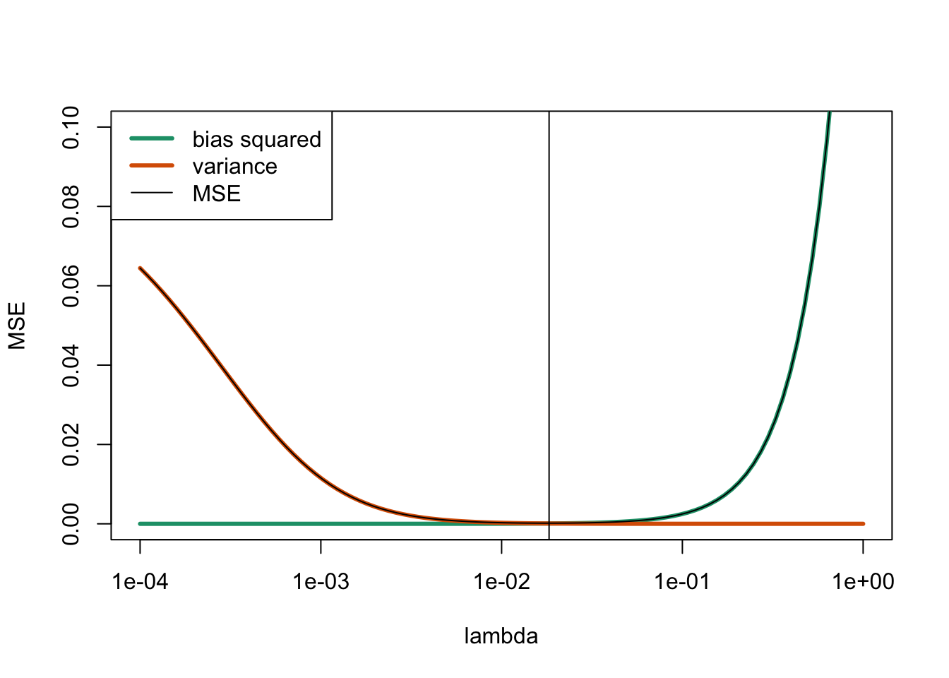
The vertical line at \(\lambda = 0.0183\) marks the optimal value of \(\lambda\). We can see that for small \(\lambda\) the MSE is dominated by the variance, whereas for large \(\lambda\) the main contribution is from the bias.
16.3 Standardisation
Ridge regression can be applied directly to the original data, but there are two reasons why this is often undesirable. First, the penalty term \(\|\beta\|^2\) treats all coefficients equally, which only makes sense if they have similar magnitudes. Second, the results would depend on the arbitrary choice of units for each predictor. Both issues are resolved by standardising the predictors before fitting the model: this ensures the penalty applies equally to all coefficients and makes the method independent of measurement units. The results can then be transformed back to obtain \(\hat{y}\) on the original scale.
We standardise every column of the input separately: For the input variable \(x_j\), where \(j\in\{1, \ldots, p\}\), we get \[\begin{equation*} w_{ij} := \frac{x_{ij} - \overline{x_j}}{\mathrm{s}_{x_j}}, \end{equation*}\] for all \(i \in \{1, \ldots, n\}\), where \(\overline{x_j} = \frac1n \sum_{i=1}^n x_{ij}\) and \[\begin{equation*} \mathrm{s}_{x_j}^2 = \frac{1}{n-1} \sum_{i=1}^n (x_{ij} - \overline{x_j})^2 \end{equation*}\] is the sample variance. We similarly standardise the outputs: \[\begin{equation*} z_i := \frac{y_i - \overline{y}}{\mathrm{s}_y}, \end{equation*}\] where \(\overline{y}\) and \(\mathrm{s}_y\) are the mean and standard deviation of the \(y_i\). If we denote the regression coefficients for the transformed data by \(\gamma\), then the residual sum of squares for the transformed data is \[\begin{equation*} r_\mathrm{tfm}(\gamma) = \sum_{i=1}^n \bigl(z_i - \gamma_0 - \gamma_1 w_{i1} - \cdots - \gamma_p w_{ip} \bigr)^2. \end{equation*}\]
The transformed inputs satisfy \[\begin{equation*} \sum_{i=1}^n w_{ij} = 0 \end{equation*}\] for all \(j\in\{1, \ldots, p\}\) and a similar relation holds for the output. Using these relations we find \[\begin{align*} r_\mathrm{tfm}(\gamma) &= \sum_{i=1}^n \Bigl( \bigl( z_i - \gamma_1 w_{i1} - \cdots - \gamma_p w_{ip} \bigr)^2 \Bigr. \\ &\hskip2cm \Bigl. - 2 \gamma_0 \bigl( z_i - \gamma_1 w_{i1} - \cdots - \gamma_p w_{ip} \bigr) + \gamma_0^2 \Bigr) \\ &= \sum_{i=1}^n \bigl( z_i - \gamma_1 w_{i1} - \cdots - \gamma_p w_{ip} \bigr)^2 \\ &\hskip2cm - 2 \gamma_0 \sum_{i=1}^n \bigl( z_i - \gamma_1 w_{i1} - \cdots - \gamma_p w_{ip} \bigr) + n \gamma_0^2 \\ &= \sum_{i=1}^n \bigl( z_i - \gamma_1 w_{i1} - \cdots - \gamma_p w_{ip} \bigr)^2 \\ &\hskip2cm - 2 \gamma_0 \Bigl( \sum_{i=1}^n z_i - \gamma_1 \sum_{i=1}^n w_{i1} - \cdots - \gamma_p \sum_{i=1}^n w_{ip} \Bigr) + n \gamma_0^2 \\ &= \sum_{i=1}^n \bigl( z_i - \gamma_1 w_{i1} - \cdots - \gamma_p w_{ip} \bigr)^2 + n \gamma_0^2. \end{align*}\] Thus, the coefficient for the intercept can be minimised separately and the optimal value is always \(\gamma_0 = 0\). The same argument applies to ridge regression: adding the penalty term \(\lambda \|\gamma\|^2 = \lambda (\gamma_0^2 + \gamma_1^2 + \cdots + \gamma_p^2)\) replaces \(n \gamma_0^2\) by \((n + \lambda) \gamma_0^2\), but this term is still independent of the other coefficients and is minimised by \(\gamma_0 = 0\). For this reason we do not include the intercept in our model for the standardised data. The design matrix is thus \[\begin{equation*} W = \begin{pmatrix} w_{1,1} & \cdots & w_{1,p} \\ w_{2,1} & \cdots & w_{2,p} \\ \vdots & \ddots & \vdots \\ w_{n,1} & \cdots & w_{n,p} \end{pmatrix} \in \mathbb{R}^{n\times p}, \end{equation*}\] and the reduced coefficient vector is \(\gamma \in \mathbb{R}^p\). The least squares estimator for the transformed data is then given by \[\begin{equation*} \hat\gamma = (W^\top W)^{-1} W^\top z \end{equation*}\] and the ridge regression estimate is given by \[\begin{equation*} \hat\gamma^{(\lambda)} = (W^\top W + \lambda I)^{-1} W^\top z. \end{equation*}\]
To transform back regression estimates obtained for the transformed data, we need to revert the standardisation: we have \[\begin{equation*} x_{ij} = \mathrm{s}_{x_j} w_{ij} + \overline{x_j} \end{equation*}\] and \[\begin{equation*} y_i = \mathrm{s}_y z_i + \overline{y}. \end{equation*}\] To obtain fitted values for an input \((\tilde x_1, \ldots, \tilde x_p)\) we have to first transform these inputs: \(\tilde w_j = (\tilde x_j - \overline{x_j}) / \mathrm{s}_{x_j}\). Note that the mean and standard deviation come from the data used to fit the model, and are not computed from the \(\tilde x_i\). We then find the model mean for the transformed data: \[\begin{align*} \hat z &= \sum_{j=1}^p \hat\gamma_j \tilde w_j \\ &= \sum_{j=1}^p \hat\gamma_j \frac{\tilde x_j - \overline{x_j}}{\mathrm{s}_{x_j}} \\ &= - \sum_{k=1}^p \frac{1}{\mathrm{s}_{x_k}} \hat\gamma_k \overline{x_k} + \sum_{j=1}^p \frac{1}{\mathrm{s}_{x_j}} \hat\gamma_j \tilde x_j. \end{align*}\] Finally, transforming back the response we get \[\begin{align*} \hat y &= \bigl( \overline{y} - \sum_{k=1}^p \frac{\mathrm{s}_y}{\mathrm{s}_{x_k}} \hat\gamma_k \overline{x_k} \bigr) + \sum_{j=1}^p \frac{\mathrm{s}_y}{\mathrm{s}_{x_j}} \hat\gamma_j \tilde x_j \\ &= \hat\beta_0 + \sum_{j=1}^p \hat\beta_j \tilde x_j, \end{align*}\] where \[\begin{equation*} \hat\beta_j = \frac{\mathrm{s}_y}{\mathrm{s}_{x_j}} \hat\gamma_j \end{equation*}\] for all \(j \in \{1, \ldots, p\}\) and \[\begin{equation*} \hat\beta_0 = \overline{y} - \sum_{k=1}^p \frac{\mathrm{s}_y}{\mathrm{s}_{x_k}} \hat\gamma_k \overline{x_k} = \overline{y} - \sum_{k=1}^p \hat\beta_k \overline{x_k}. \end{equation*}\] This transformation can be used both for least squares regression and ridge regression estimates.
This section concludes our discussion about using linear regression in practice. In the remaining part of these notes we will discuss how to perform linear regression in the presence of outliers.
Summary
- Ridge regression is an alternative estimator for the regression coefficients.
- The method is useful when multicollinearity is present.
- Ridge regression is biased, but can achieve lower mean squared error than least squares by reducing variance.
- It is advantageous to standardise the data before performing ridge regression.