Problem Sheet 5
You should attempt all these questions and write up your solutions in advance of the workshop in week 11 where the answers will be discussed.
17. Consider the dataset at
which contains samples from variables \(x_1, x_2, y \in \mathbb{R}\) and \(x_3 \in \{\mathrm{R}, \mathrm{G}, \mathrm{B}\}\).
- Load the data into R.
We can load the data into R as follows:
# data from https://teaching.seehuhn.de/2022/MATH3714/
dd <- read.csv("data/P05Q17.csv")
# fix the order of levels:
dd$x3 <- factor(dd$x3, levels = c("R", "G", "B"))
head(dd)
x1 x2 x3 y
1 1.940066 -0.7755552 B 2.709368
2 -1.214413 0.4842872 R 1.254138
3 1.940301 3.1189902 B 3.228220
4 4.599154 3.5881714 B 5.541995
5 3.891628 -4.4026497 B 4.018021
6 2.615079 -0.9916691 R 0.449100- Fit a simple linear model to describe \(y\) as a function of \(x_1\), \(x_2\) and \(x_3\), taking into account that \(x_3\) is a categorical variable. Show that the behaviour of the residuals depends on the levels of \(x_3\).
To fit a simple linear model:
Call:
lm(formula = y ~ ., data = dd)

Residuals:
    Min      1Q  Median      3Q     Max
-2.7641 -1.0211  0.0354  0.6991  3.7245

Coefficients:
            Estimate Std. Error t value Pr(>|t|)
(Intercept)  0.91712    0.37429   2.450   0.0182 *
x1           0.51294    0.07220   7.105 7.13e-09 ***
x2           0.53629    0.08328   6.440 6.93e-08 ***
x3G          0.10016    0.57361   0.175   0.8622
x3B         -0.25865    0.51595  -0.501   0.6186
---
Signif. codes:  0 '***' 0.001 '**' 0.01 '*' 0.05 '.' 0.1 ' ' 1

Residual standard error: 1.54 on 45 degrees of freedom
Multiple R-squared:  0.7044,    Adjusted R-squared:  0.6781
F-statistic:  26.8 on 4 and 45 DF,  p-value: 2.082e-11
In a residual plot we can colour-code the residuals by the level of \(x_3\):
plot(fitted(m), resid(m),
     col = as.numeric(dd$x3) + 1, pch = as.numeric(dd$x3) + 1)
legend("topleft", legend = levels(dd$x3), col=2:4, pch = 2:4)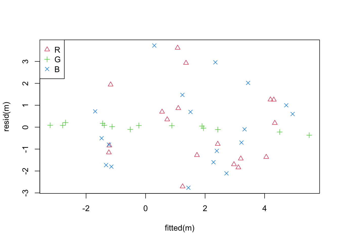
This shows that that the residuals for level G are much smaller
than for the other levels.
- Find an improved model, which includes some of the interaction terms between \(x_3\) and the other variables. For each level of \(x_3\), write the mathematical equation for the fitted model mean of your chosen model.
We can start by trying all interaction terms:
Call:
lm(formula = y ~ .^2, data = dd)

Residuals:
      Min        1Q    Median        3Q       Max
-0.139522 -0.058383 -0.002396  0.037826  0.227631

Coefficients:
              Estimate Std. Error t value Pr(>|t|)
(Intercept)  1.0129619  0.0216220  46.849   <2e-16 ***
x1           0.1017179  0.0069591  14.617   <2e-16 ***
x2           0.8860760  0.0073076 121.254   <2e-16 ***
x3G         -0.0287990  0.0334521  -0.861    0.394
x3B          0.0082008  0.0300303   0.273    0.786
x1:x2       -0.0007807  0.0016391  -0.476    0.636
x1:x3G       0.4025315  0.0125449  32.087   <2e-16 ***
x1:x3B       0.8029663  0.0088744  90.481   <2e-16 ***
x2:x3G      -0.3936519  0.0131191 -30.006   <2e-16 ***
x2:x3B      -0.7841714  0.0105136 -74.586   <2e-16 ***
---
Signif. codes:  0 '***' 0.001 '**' 0.01 '*' 0.05 '.' 0.1 ' ' 1

Residual standard error: 0.08068 on 40 degrees of freedom
Multiple R-squared:  0.9993,    Adjusted R-squared:  0.9991
F-statistic:  6160 on 9 and 40 DF,  p-value: < 2.2e-16
Many of the interaction terms are significantly
different from zero and the adjusted \(R^2\)-value has
dramatically increased. A good choice of model seems
to be y ~ x1 + x2 + x1:x3 + x2:x3
Call:
lm(formula = y ~ x1 + x2 + x1:x3 + x2:x3, data = dd)

Residuals:
      Min        1Q    Median        3Q       Max
-0.136497 -0.053054 -0.003199  0.040097  0.241331

Coefficients:
             Estimate Std. Error t value Pr(>|t|)
(Intercept)  1.006764   0.012370   81.39   <2e-16 ***
x1           0.101630   0.006318   16.09   <2e-16 ***
x2           0.886702   0.006935  127.86   <2e-16 ***
x1:x3G       0.404014   0.012109   33.37   <2e-16 ***
x1:x3B       0.803071   0.008462   94.91   <2e-16 ***
x2:x3G      -0.392663   0.012882  -30.48   <2e-16 ***
x2:x3B      -0.783259   0.009569  -81.85   <2e-16 ***
---
Signif. codes:  0 '***' 0.001 '**' 0.01 '*' 0.05 '.' 0.1 ' ' 1

Residual standard error: 0.08005 on 43 degrees of freedom
Multiple R-squared:  0.9992,    Adjusted R-squared:  0.9991
F-statistic:  9383 on 6 and 43 DF,  p-value: < 2.2e-16
The fitted model mean for \(x_3 = \mathrm{R}\) is \[\begin{equation*} y \approx 1.007 + 0.102 x_1 + 0.887 x_2. \end{equation*}\] For \(x_3 = \mathrm{G}\) we get \[\begin{align*} y &\approx 1.007 + (0.102 + 0.404) x_1 + (0.887 - 0.393) x_2 \\ &= 1.007 + 0.506 x_1 + 0.494 x_2 \end{align*}\] Finally, for \(x_3 = \mathrm{B}\) we find \[\begin{align*} y &\approx 1.007 + (0.102 + 0.803) x_1 + (0.887 - 0.783) x_2 \\ &= 1.007 + 0.905 x_1 + 0.104 x_2. \end{align*}\]
18. Consider the dataset at
Identify the \(x\)-space outlier in this dataset.
We start by loading the data into R:
            x1          x2         x3         x4
1 -1.359560124  0.66310168  2.5866758 -1.7229394
2  0.624644511 -0.01925607 -0.1692926 -0.5092775
3  0.957938698 -0.54734504 -0.9680673  0.6074693
4  0.733255177 -0.37217623 -0.6027061  0.2751777
5  0.355021570 -0.58332351  0.2386221 -0.1934059
6  0.002907357 -0.69562237  0.5365051  0.3047116
To identify the outlier, we compute the leverage of each sample.
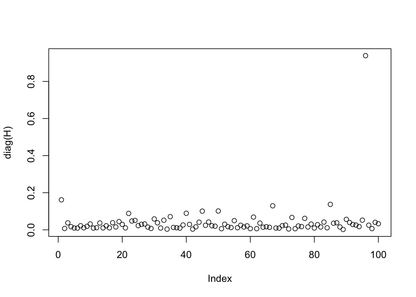
The plot shows that one sample has a much larger leverage than the other samples.
[1] 96Thus, the \(x\)-space outlier is in row 96 of the matrix \(X\).
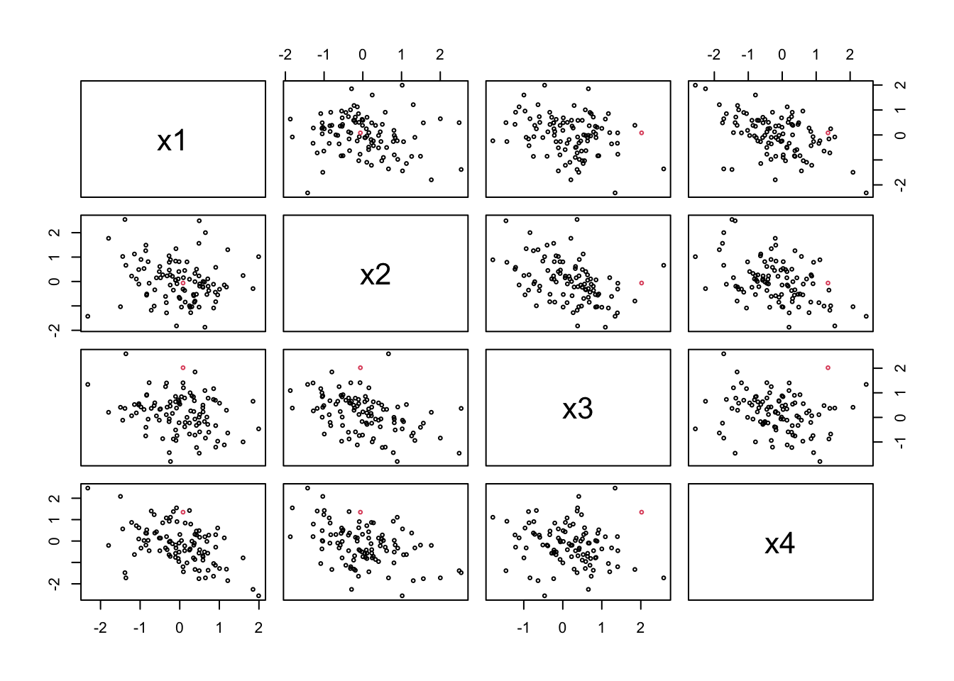
Note that the outlier does not look special on a pair scatter plot:
19. The sample median is a robust estimator of the mean. Determine the breakdown point.
The median can be obtained by arranging the samples in increasing order and inspecting the middle element (for odd \(n\)) or the middle two elements (for even \(n\)) in this list. Let \(x_{(1)}, \ldots, x_{(n)}\) be the samples arranged in increasing order.
For odd \(n\): The median equals \(x_{(k)}\) where \(k = (n+1) / 2\). In order to move the median to infinity, we have to move \(x_{(k)}, x_{(k+1)}, \ldots, x_{(n)}\) to infinity. These are \((n+1) / 2\) values in total and thus the breakdown point is \((n+1) / 2n\).
For even \(n\): The median equals \((x_{(k)} + x_{(k+1)})/2\) where \(k = n / 2\). In order to move the median to infinity, we have to move \(x_{(k+1)}, x_{(k+2)}, \ldots, x_{(n)}\) to infinity. These are \(n / 2\) values in total and thus the breakdown point is \(1/2\).
20. Determine the breakdown point for the resistant line from example 17.3.
The regression coefficients in the example are computed as \[\begin{equation*} \hat\beta_1 = \frac{y_\mathrm{R} - y_\mathrm{L}}{x_\mathrm{R} - x_\mathrm{L}} \end{equation*}\] and \[\begin{equation*} \hat\beta_0 = \frac{y_\mathrm{L} + y_\mathrm{M} + y_\mathrm{R}}{3} - \hat\beta_1 \frac{x_\mathrm{L} + x_\mathrm{M} + x_\mathrm{R}}{3}, \end{equation*}\] where \(x_\mathrm{L}\), \(x_\mathrm{M}\) and \(x_\mathrm{R}\) are the medians of the lower, middle and upper third of the \(x_{(i)}\), and \(y_\mathrm{L}\), \(y_\mathrm{M}\) and \(y_\mathrm{R}\) are the medians of the corresponding \(y\) values, respectively.
To move either of the estimated regression coefficients to infinity, we need to move one of \(x_\mathrm{L}\), \(x_\mathrm{M}\), \(x_\mathrm{R}\), \(y_\mathrm{L}\), \(y_\mathrm{M}\), or \(y_\mathrm{R}\) to infinity. From the previous question we know that this requires to modify half of the corresponding third of the data, so the breakdown point of the method is \(1/2 \cdot 1/3 = 1/6\).