Section 13 Exhaustive Model Search
13.1 Exhaustive Search
The stepwise methods from the previous section provide efficient heuristics, but they may not find the model with truly maximal \(R^2_\mathrm{adj}\). When \(p\) is small to moderate, exhaustive search allows us to evaluate all possible models systematically. Here we present an efficient algorithm that can often find the optimal model without having to fit all \(2^p\) models. We consider the least squares estimate throughout.
We can characterise each possible model by the set \(J \subseteq \{1, \ldots p\}\) of variables included in the model. The model includes variable \(x_j\), if and only if \(j \in J\). Here we assume that the intercept is always included, so that \(J=\emptyset\) corresponds to the model \(Y = \beta_0 + \varepsilon\).
The method described in this section is based on the following three observations:
In order to maximise \(R^2_\mathrm{adj}\), we can equivalently also find the \(J\) which minimises \[\begin{equation*} \hat\sigma^2(J) := \frac{1}{n - |J| - 1} \sum_{i=1}^n (y_i - \hat y_i)^2, \end{equation*}\] where \(|J|\) is the number of variables in \(J\) and the \(\hat y_i\) are the fitted values for the model with inputs \(j \in J\). We have seen in 10.3 that these criteria are equivalent.
For \(J \subseteq \{1, \ldots p\}\), define \[\begin{equation*} r(J) := \sum_{i=1}^n (y_i - \hat y_i)^2 \end{equation*}\] where \(\hat y_i\) are the fitted values for the model corresponding to \(J\). This gives the residual sum of squares for each model. Then we have \[\begin{align*} \min_J \hat\sigma^2(J) &= \min_J \frac{1}{n - |J| - 1} \sum_{i=1}^n (y_i - \hat y_i)^2 \\ &= \min_{q \in \{0, 1, \ldots, p\}} \min_{J, |J|=q} \frac{1}{n - q - 1} r(J) \\ &= \min_{q \in \{0, 1, \ldots, p\}} \frac{1}{n - q - 1} \min_{J, |J|=q} r(J). \end{align*}\] This means that we can first minimise the residual sum of squares for each fixed number \(q\) of inputs, and then find the \(q\) which gives the best \(\hat\sigma^2\) in a second step.
Adding a variable never increases the residual sum of squares. Thus we have \(r(J) \leq r(K)\) whenever \(J \supseteq K\). We can use this result to exclude certain models without having to fit them.
13.2 Search Algorithm
To find the model with optimal adjusted R-squared value, we perform the following steps. The algorithm is based on the ideas explained in the previous section.
Let \(\varphi_j\) denote the residual sum of squares for the model containing all variables except \(x_j\): \[\begin{equation*} \varphi_j := r\bigl( \{ 1, \ldots, p \} \setminus \{ j \} \bigr). \end{equation*}\] Suppose that the \(x_j\) are ordered so that \[\begin{equation*} \varphi_1 \geq \varphi_2 \geq \cdots \geq \varphi_p. \end{equation*}\] Any model \(J\) with \(j \notin J\) has \(r(J) \geq \varphi_j\).
Compute \(\min_{J, |J|=0} r(J) = r(\emptyset)\). This is the residual sum of squares of the model which consists only of the intercept.
For each \(q := 1, \ldots, p-2\):
Let \[\begin{equation*} r := r\bigl( \{1, \ldots, q\} \bigr). \end{equation*}\] This is the only model with \(q\) inputs where the first excluded variable has index \(k = q+1\). If \(r \leq \varphi_{k-1} = \varphi_q\), we know from step A that \(J = \{1, \ldots, q\}\) is the best model with \(q\) inputs, since any other model will exclude one of the \(x_j\) with \(j \leq q\). In this case we have found \[\begin{equation*} \min_{J, |J|=q} r(J) = r. \end{equation*}\] and we continue step C by trying the next value of \(q\). If \(r > \varphi_{k-1}\), no decision can be taken at this point and we continue with step 2.
For \(j \in \{q+1, \ldots, p\}\) let \[\begin{equation*} r_j := r\bigl( \{1, \ldots, q-1\} \cup \{j\} \bigr). \end{equation*}\] These are all models with \(q\) inputs where the first excluded variable has index \(k = q\). If \(\min(r, r_{q+1}, \ldots, r_p) \leq \varphi_{k-1} = \varphi_{q-1}\), then we know from step A that the \(J\) corresponding to the minimum is the best model with \(q\) inputs. In this case we continue step C by trying the next value of \(q\). Otherwise we proceed to step 3.
Similarly to the previous step, we consider all models with \(q\) variables where the first excluded variable has index \(k = q-1\). If the best RSS amongst these and the previously considered models is less than or equal to \(\varphi_{k-1}\) we are done and consider the next \(q\). Otherwise we decrease \(k\) until we reach \(k = 1\). At this point we have considered all models with \(q\) variables and have found \(\min_{J, |J|=q} r(J)\).
Compute \(\min_{J, |J|=p-1} r(J) = \min_{j \in \{1, \ldots, p\}} \varphi_j\).
Compute \(\min_{J, |J|=p} r(J) = r\bigl( \{1, \ldots, p\} \bigr)\).
Find the \(q \in \{0, \ldots, p\}\) for which \(\min_{J, |J|=q} r(J) / (n-q-1)\) is smallest. Output the model which has minimal RSS for this \(q\).
This algorithm finds the model with the maximal \(R^2_\mathrm{adj}\). Often, large savings are achieved by the early exits in step C. Only in the worst case, when all of the comparisons with \(\varphi_j\) in step C fail, this algorithm needs to fit all \(2^p\) models.
Example 13.1 To demonstrate the steps of the algorithm, we implement the method “by hand”. We use the QSAR dataset, which we have already seen in section 7:
# data from https://archive.ics.uci.edu/ml/datasets/QSAR+aquatic+toxicity
qsar <- read.csv("data/qsar_aquatic_toxicity.csv",
                 sep = ";", header = FALSE)
fields <- c(
    "TPSA",
    "SAacc",
    "H050",
    "MLOGP",
    "RDCHI",
    "GATS1p",
    "nN",
    "C040",
    "LC50"
)
names(qsar) <- fields
To make it easy to add/remove columns automatically, we first construct
the design matrix, remove columns as needed, and then use the resulting
matrix in the call to lm() (instead of specifying the terms to include
by name).
X <- model.matrix(LC50 ~ ., data = qsar)
X <- X[, -1] # remove the intercept, since lm() will re-add it later
n <- nrow(X)
p <- ncol(X)

y <- qsar$LC50

m <- lm(y ~ X) # full model
summary(m)
Call:
lm(formula = y ~ X)

Residuals:
    Min      1Q  Median      3Q     Max
-4.4934 -0.7579 -0.1120  0.5829  4.9778

Coefficients:
             Estimate Std. Error t value Pr(>|t|)
(Intercept)  2.698887   0.244554  11.036  < 2e-16 ***
XTPSA        0.027201   0.002661  10.220  < 2e-16 ***
XSAacc      -0.015081   0.002091  -7.211 1.90e-12 ***
XH050        0.040619   0.059787   0.679 0.497186
XMLOGP       0.446108   0.063296   7.048 5.60e-12 ***
XRDCHI       0.513928   0.135565   3.791 0.000167 ***
XGATS1p     -0.571313   0.153882  -3.713 0.000227 ***
XnN         -0.224751   0.048301  -4.653 4.12e-06 ***
XC040        0.003194   0.077972   0.041 0.967340
---
Signif. codes:  0 '***' 0.001 '**' 0.01 '*' 0.05 '.' 0.1 ' ' 1

Residual standard error: 1.203 on 537 degrees of freedom
Multiple R-squared:  0.4861,    Adjusted R-squared:  0.4785
F-statistic:  63.5 on 8 and 537 DF,  p-value: < 2.2e-16
Comparing the output to what we have seen in section 7
shows that the new method of calling lm() gives the same results
as before. Now we follow the steps of the algorithm.
A. The values \(\varphi_1, \ldots, \varphi_p\) can be computed as follows:
phi <- numeric(p) # pre-allocate an empty vector
for (j in 1:p) {
    idx <- (1:p)[-j] # all variables except x[j]
    m <- lm(y ~ X[,idx])
    phi[j] <- sum(resid(m)^2)
}

# change the order of columns in X, so that the phi_j are decreasing
jj <- order(phi, decreasing = TRUE)
X <- X[, jj]
phi <- phi[jj]
plot(phi, xlab = "j", ylab = expression(varphi[j]))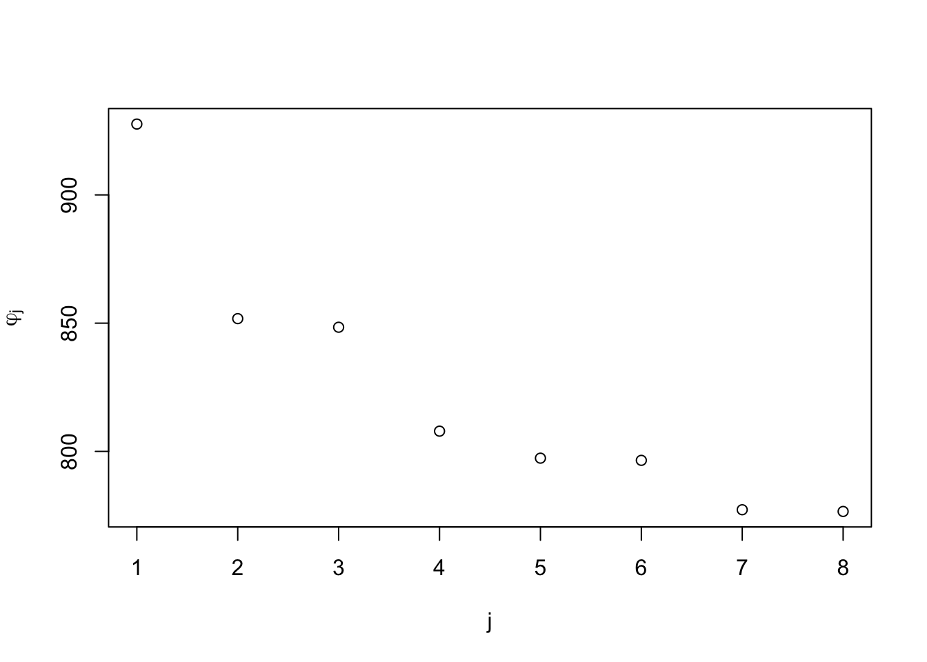
The plot shows the residual sum of squares for the model with input \(x_j\) omitted, for \(j\) ranging from 1 to 8.
B. Next, we compute the residual sum of squares of the model which consists only of the intercept. This is the case \(q = 0\).
all.q <- 0:p
best.rss <- numeric(p + 1) # For storing the best RSS for q = 0, ..., p,
best.model <- vector("list", p + 1) # and the corresponding models.

m <- lm(y ~ 1)
best.rss[0 + 1] <- sum(resid(m)^2)
best.model[[0 + 1]] <- integer(0) # a vector of length 0 (no columns)

count <- 1 # number of models fitted so far
C. Now we consider \(q \in \{1, \ldots, p-2\}\). The algorithm groups
these cases by the position \(k\) of the first column omitted in the model,
starting with \(k = q+1\) and then decreasing \(k\) in each step.
We use the function combn to get all possible choices of
\(q - k + 1\) columns out of \(\{k+1, \ldots, p\}\).
for (q in 1:(p-2)) {
    best.rss[q + 1] <- Inf

    # Consider all sets of q columns, ...
    for (k in (q+1):1) {
        # ... where the first omitted column is k.

        # We have to include 1, ..., k-1, and ...
        a <- seq_len(k-1)

        # ... for the remaining q - (k-1) inputs, we try all
        # possible combinations.
        bb <- combn((k+1):p, q - k + 1)
        for (l in seq_len(ncol(bb))) {
            b <- bb[, l]
            included <- c(a, b)

            m <- lm(y ~ X[, included])
            count <- count + 1
            rss <- sum(resid(m)^2)

            if (rss < best.rss[q + 1]) {
                best.rss[q + 1] <- rss
                best.model[[q + 1]] <- included
            }
        }

        if (k > 1 && best.rss[q+1] <= phi[k-1]) {
            # If we reach this point, we know that we found the best
            # arrangement and we can exit the loop over k early.
            # This is what makes the algorithm efficient.
            break
        }
    }
}
D. We already fitted all models with \(p-1\) inputs, when we computed phi.
Since we sorted the models, the best of these models is last in the list.
This covers the case \(q = p - 1\).
best.rss[(p - 1) + 1] <- min(phi)
omitted <- jj[length(jj)]
best.model[[(p - 1) + 1]] <- (1:p)[-omitted]
count <- count + length(phi)
E. Finally, for \(q = p\) we fit the full model:
F. Now we can find the model with the best \(R^2_\mathrm{adj}\):
plot(all.q, best.rss / (n - all.q - 1),
     xlab = "q", ylab = "residual variance")
best.q <- all.q[which.min(best.rss / (n - all.q - 1))]
abline(v = best.q)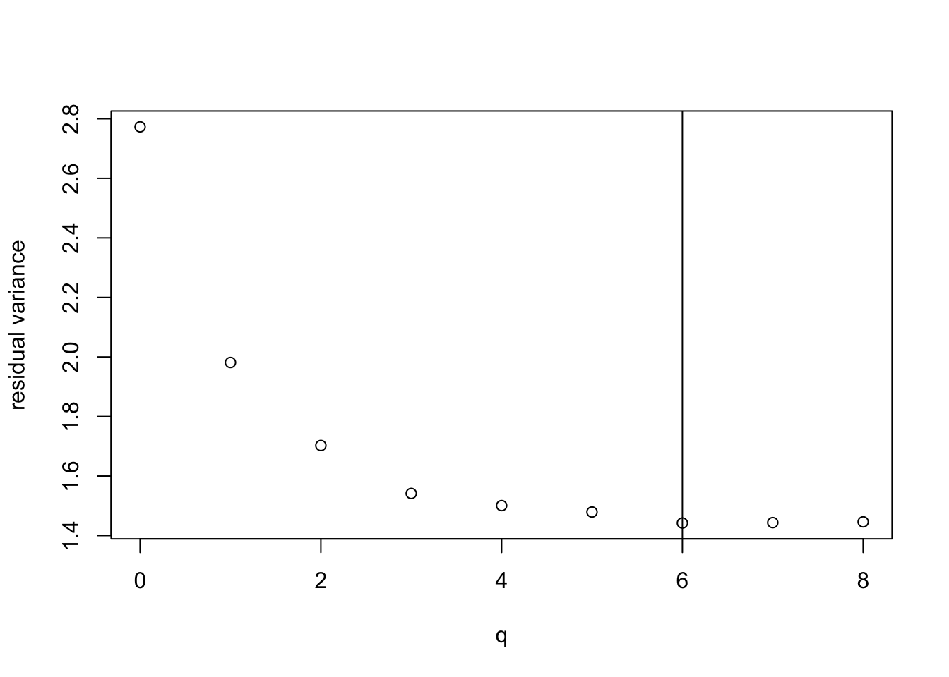
We see that the model with \(q = 6\) variables has the lowest \(\hat\sigma^2\) and thus the highest \(R^2_\mathrm{adj}\). The values for \(q = 7\) and \(q = 8\) are very close to optimal. The best model uses the following variables:
[1] "TPSA" "SAacc" "MLOGP" "nN" "RDCHI" "GATS1p"We can fit the optimal model from the original data:
Call:
lm(formula = LC50 ~ TPSA + SAacc + MLOGP + nN + RDCHI + GATS1p,
    data = qsar)

Residuals:
    Min      1Q  Median      3Q     Max
-4.4986 -0.7668 -0.1165  0.5529  4.9758

Coefficients:
             Estimate Std. Error t value Pr(>|t|)
(Intercept)  2.758246   0.228483  12.072  < 2e-16 ***
TPSA         0.026858   0.002608  10.300  < 2e-16 ***
SAacc       -0.014267   0.001660  -8.596  < 2e-16 ***
MLOGP        0.434578   0.060611   7.170 2.49e-12 ***
nN          -0.218445   0.047101  -4.638 4.43e-06 ***
RDCHI        0.514758   0.133430   3.858 0.000128 ***
GATS1p      -0.602971   0.146920  -4.104 4.69e-05 ***
---
Signif. codes:  0 '***' 0.001 '**' 0.01 '*' 0.05 '.' 0.1 ' ' 1

Residual standard error: 1.201 on 539 degrees of freedom
Multiple R-squared:  0.4857,    Adjusted R-squared:  0.4799
F-statistic: 84.82 on 6 and 539 DF,  p-value: < 2.2e-16
This shows that \(R^2_\mathrm{adj}\) has indeed marginally improved, from \(0.4785\) to \(0.4799\)
To conclude, we check that the complicated algorithm indeed saved some work:
36 models fitted (14.1%)This shows that we only needed to fit 88 of the 256 models under consideration.
Example 13.2 We can perform the analysis from the previous example automatically,
using the function regsubsets() from the leaps package:
Subset selection object
Call: regsubsets.formula(LC50 ~ ., data = qsar, method = "exhaustive")
8 Variables  (and intercept)
       Forced in Forced out
TPSA       FALSE      FALSE
SAacc      FALSE      FALSE
H050       FALSE      FALSE
MLOGP      FALSE      FALSE
RDCHI      FALSE      FALSE
GATS1p     FALSE      FALSE
nN         FALSE      FALSE
C040       FALSE      FALSE
1 subsets of each size up to 8
Selection Algorithm: exhaustive
         TPSA SAacc H050 MLOGP RDCHI GATS1p nN  C040
1  ( 1 ) " "  " "   " "  "*"   " "   " "    " " " "
2  ( 1 ) "*"  " "   " "  "*"   " "   " "    " " " "
3  ( 1 ) "*"  "*"   " "  "*"   " "   " "    " " " "
4  ( 1 ) "*"  "*"   " "  "*"   " "   " "    "*" " "
5  ( 1 ) "*"  "*"   " "  "*"   " "   "*"    "*" " "
6  ( 1 ) "*"  "*"   " "  "*"   "*"   "*"    "*" " "
7  ( 1 ) "*"  "*"   "*"  "*"   "*"   "*"    "*" " "
8  ( 1 ) "*"  "*"   "*"  "*"   "*"   "*"    "*" "*"
This shows the best model of each size. The only step left is to decide which \(q\) to use. This choice depends on the cost-complexity tradeoff. Here we consider \(R^2_\mathrm{adj}\) again:
[1] 0.2855 0.3860 0.4441 0.4588 0.4666 0.4799 0.4795 0.4785This gives the \(R^2_\mathrm{adj}\) for the optimal model of each size
again. At the end of the list we recognise the values 0.4799 and
0.4785 from our previous analysis.
Remark. Like stepwise methods, exhaustive search is affected by using the same data for both model selection and inference: test statistics and confidence intervals from the selected model are biased and overly optimistic. Validation on independent data is advisable.
This concludes our discussion of model selection techniques. In the next section we turn to a new topic: how to include categorical variables (called factors) in regression models.
Summary
- Exhaustive search finds the model with truly maximal \(R^2_\mathrm{adj}\), unlike stepwise heuristics which may miss the optimal combination.
- An efficient algorithm can find the optimal model without fitting all \(2^p\) models, by using algebraic properties of the residual sum of squares.
- The
regsubsets()function from theleapspackage implements this algorithm in R. - For very large \(p\), even exhaustive search becomes infeasible, and stepwise methods remain the practical choice.