Section 20 Examples

In this section we compare the robust regression methods from sections 17, 18 and 19 by applying them to synthetic data. We will see how methods with different breakdown points behave in the presence of outliers, how the weights assigned by different M-estimators differ in practice, and how robust methods produce cleaner residual patterns than least squares regression.

20.1 Comparing Robust Methods

Example 20.1 We compare several robust estimators on a synthetic dataset with outliers. This example illustrates how methods with high breakdown points resist contamination, whilst methods with low breakdown points can be severely affected.

We start by generating data from a linear relationship with three outliers:

set.seed(20251006)

n <- 30
x <- runif(n, 0, 10)
y <- 2 + 0.5*x + rnorm(n, sd = 0.5)

# Add three contaminants:
outliers <- c(5, 15, 25)
x[outliers] <- c(9.5, 10, 10.5)
y[outliers] <- c(-2.5, -3, -3.5)

Now we fit several different regression methods to this data:

library(MASS)     # for rlm() and lqs()
library(quantreg) # for rq()

Loading required package: SparseM

lm1   <- lm(y ~ x)                           # LSQ
rq1   <- rq(y ~ x)                           # LAV
rlm1  <- rlm(y ~ x, psi = psi.huber)         # Huber
rlm2  <- rlm(y ~ x, psi = psi.bisquare)      # Bisquare
rlm3  <- rlm(y ~ x, psi = psi.hampel)        # Hampel
lms1  <- lqs(y ~ x, method = "lms")          # LMS
lts1  <- lqs(y ~ x, method = "lts")          # LTS

The left plot in figure 20.1 shows the fitted lines from all seven methods. As expected, only those methods with high breakdown point (LMS and LTS) have resisted the gross outliers. The least squares, LAV and M-estimator lines all pass between the bulk of the data and the outliers, demonstrating their susceptibility to contamination.

The right plot shows how the LTS estimator behaves for different values of the parameter \(k\) (called quantile in R). For smaller values of \(k\), the method uses only the observations with smallest residuals and has higher breakdown point. As \(k\) increases towards \(n = 30\), the method gradually converges to the least squares estimate.

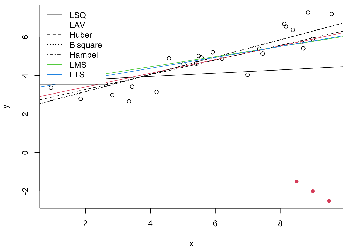
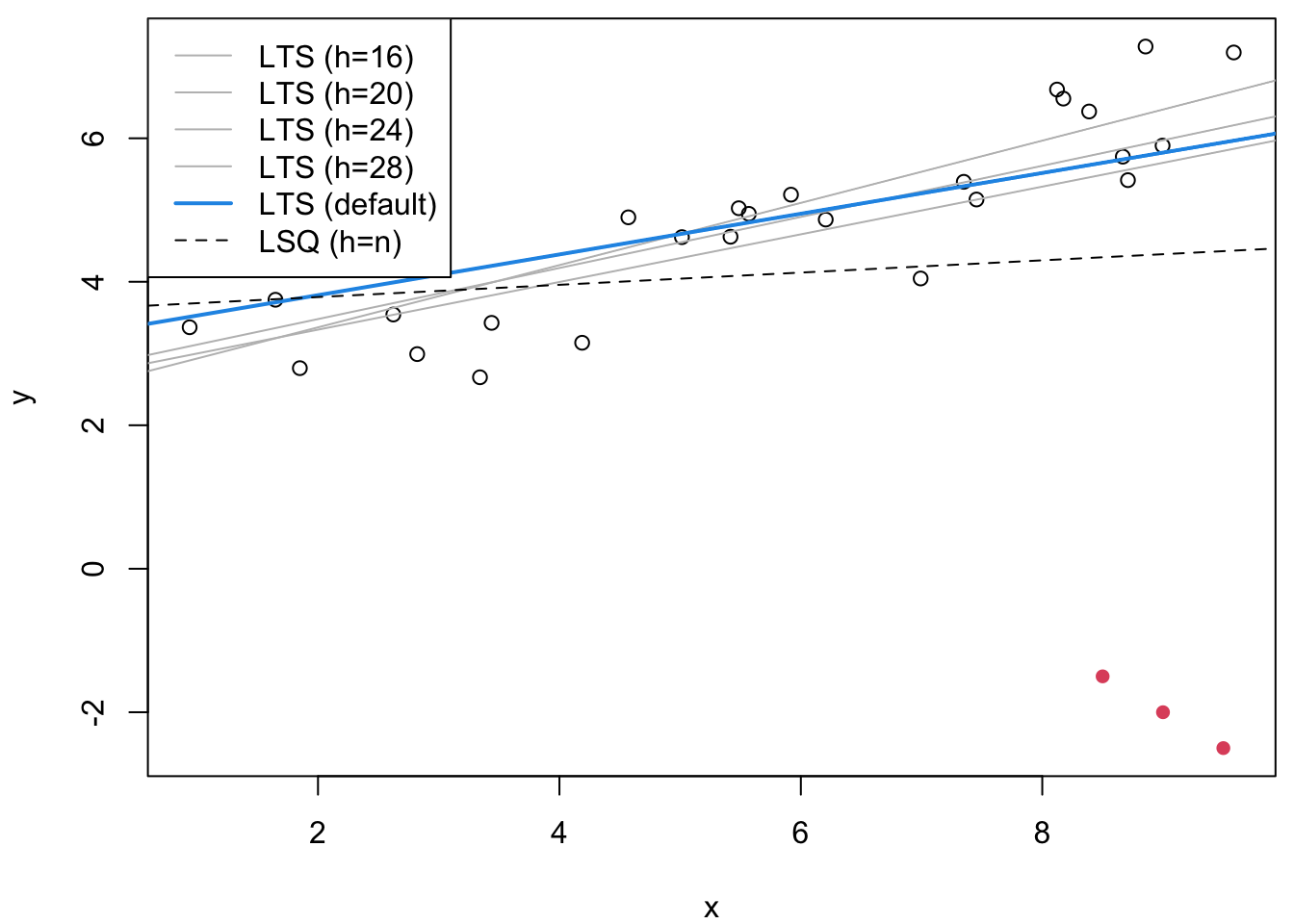
Figure 20.1: On the left we compare several methods. As expected, only those with high breakdown point have resisted the outliers. On the right plot, we compare different values of the parameter \(k\) for the LTS estimator.

We see that for small \(k\) the LTS line passes through the bulk of the data and ignores the outliers, whilst for larger \(k\) it is increasingly influenced by the outliers until it converges to the least squares line.

20.2 Residual Analysis

Example 20.2 Continuing with the same dataset, we now examine the residual patterns from different methods. When outliers influence the fitted line, the residuals from the remaining observations often exhibit systematic patterns.

Figure 20.2 shows the residuals from three methods, excluding the three known outliers. The least squares residuals (left plot) show a clear trend. This pattern indicates that the outliers have pulled the regression line away from the bulk of the data.

The LAV and Huber methods (centre and right plots) show much less pronounced patterns. The residuals are more evenly scattered around zero, indicating that these methods have been less influenced by the outliers. This demonstrates one advantage of robust methods: they not only provide better parameter estimates in the presence of outliers, but also produce more reliable residual plots for model diagnostics.

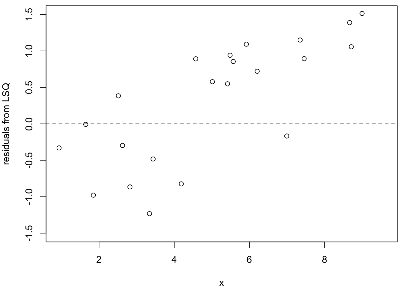
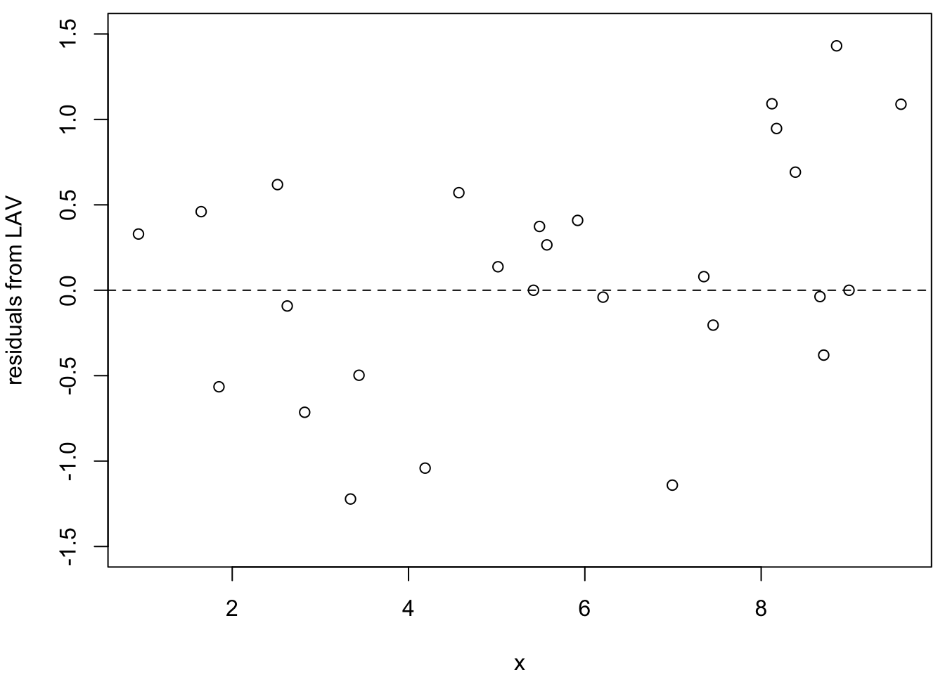
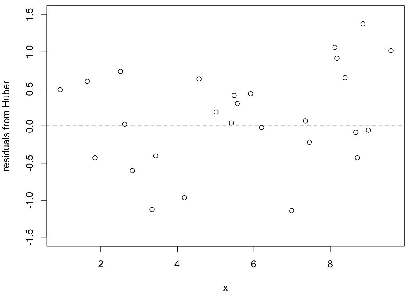
Figure 20.2: Residuals from non-outlier observations for three methods (left: LSQ; centre: LAV; right: Huber). The least squares residuals show a clear trend due to the influence of the outliers.

20.3 Weight Comparisons

Example 20.3 We now examine the weights assigned by different M-estimators. Recall from section 18 that M-estimators assign weights to observations based on the magnitude of their residuals, with larger residuals receiving smaller weights.

Figure 20.3 shows the weights assigned by three different M-estimators: Huber, Bisquare and Hampel. The outliers (observations 5, 15 and 25) receive low weights from all three methods, confirming that they are correctly identified as outliers. However, the methods differ in how aggressively they down-weight these observations:

• The Bisquare and Hampel methods assign zero weight to the outliers.
• The Huber method assigns intermediate weights even to the outliers, which reflects the fact that the Huber \(\psi\)-function does not completely down-weight large residuals.

These differences reflect the different shapes of the weight functions \(w(\varepsilon) = \psi(\varepsilon) / \varepsilon\) discussed in section 18. The Bisquare and Hampel methods use redescending \(\psi\)-functions, assigning zero weight to sufficiently large residuals. The Huber method uses a non-redescending \(\psi\)-function, so all observations retain some influence.

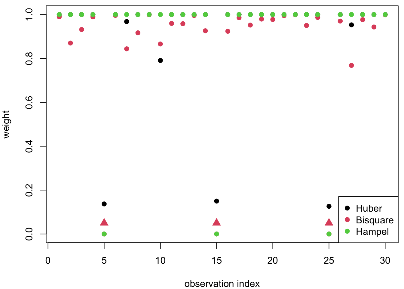
Figure 20.3: Weights assigned by three M-estimators (Huber, Bisquare, Hampel).

Summary

• M-estimators downweight outliers based on residual magnitude, producing fits that better represent the bulk of the data than least squares.
• The LTS parameter \(k\) controls how many observations contribute to the fit: smaller \(k\) gives more resistance to outliers.
• M-estimators produce cleaner residual patterns than least squares when outliers are present.
• Redescending M-estimators (Bisquare, Hampel) assign zero weight to sufficiently large residuals, whilst non-redescending M-estimators (LAV, Huber) retain some influence for all observations.