Lecture 12 Sampling Distributions and Standard Errors

The model of the day is $X_{1},\dots,X_{n}$ i.i.d. from the exponential distribution with rate $\theta$, where the maximum likelihood estimator is $\hat{\theta}=1/\bar{X}$ by example 5.2. The command rexp can be used to simulate such a sample, and as in lecture 6 we package one run as a function. Before you run the code below, predict the two histograms: for $n=10$, will the estimates form a symmetric bell around the true value $\theta=1$? Will the peak sit above, below or at $1$? How will the picture change for $n=100$?

As in lecture 9, we require the histograms to be generated with freq = FALSE and we overlay the density by using curve. The density we use is the large-sample approximation from lecture 17, which is normal with mean $\theta$ and standard deviation $\theta/\sqrt{n}$. The command qqnorm can be used to plot the sorted estimates against the quantiles of a standard normal distribution, and qqline can be used to add the line for the quantiles of a normal distribution.

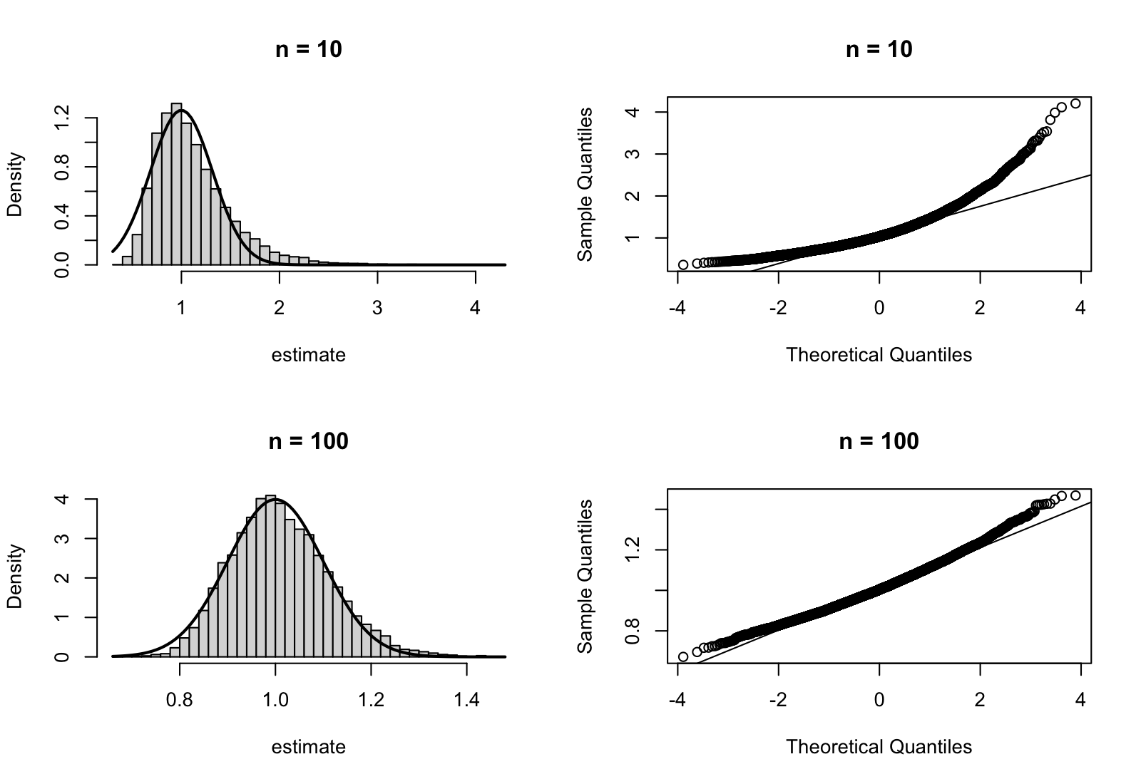
Figure 12.1 shows that for $n=10$ the estimates are not normally distributed: the histogram has a long right tail, the peak is to the left of $1$ and the quantile plot shows quantiles diverging from the line. Since $1/\bar{X}$ is not an average, the central limit theorem (theorem A.15) does not apply directly. For $n=100$ the distortion is gone: this is asymptotic normality of the maximum likelihood estimator, proved in lecture 17.

The standard deviation $\theta/\sqrt{n}$ of the normal curves in figure 12.1 is given by the Fisher information from lecture 11: By example 11.8 and definition 11.2 the sample contains information $\mathcal{I}_{n}(\theta)=n/\theta^{2}$ and lecture 17 will show that the spread of the estimator is approximately $1/\sqrt{\mathcal{I}_{n}(\theta)}=\theta/\sqrt{n}$. Normally, the value of $\theta$ is unknown and we have to evaluate the information at the estimate instead. The standard error of the estimate is given by

This is a measure of the likely size of the estimation error, computed from the data. Since the estimator is approximately normally distributed with this spread, the Wald interval $\hat{\theta}\pm 1.96\,\mathop{\mathrm{se}}\nolimits(\hat{\theta})$ covers the true value with probability approximately $95\%$. This is a confidence interval of the kind we have seen in MATH2701, and is used informally here and more formally in lecture 25. The theorem which describes the resulting recipe is corollary 17.3. Before you try the code, make a prediction: will the interval cover the true value $1$?

The interval $[0.407,0.861]$ does not contain the true value $1$. This is not a programming error: the sample happened to contain unusually large observations, and a $95\%$ interval misses the truth in about one sample out of twenty. From a single sample it is not possible to know whether this is one of the misses; how often the recipe is wrong in the long run can be answered by simulation.

The probability of an event $A$ is the expected value of the indicator of $A$, and by the law of large numbers (theorem A.14) this expectation can be approximated by the average of the indicator over many independent repetitions. In R, the mean of the logical vector abs(large - theta) <= 0.2 can be used to estimate $\mathbb{P}(|\hat{\theta}-\theta|\leq 0.2)$, since mean interprets TRUE as $1$ and FALSE as $0$. The same principle applies to all probabilities we estimate by simulation: for estimating the coverage probability of an interval, we take the average of the indicator that the interval contains the truth. Similarly, the rejection rate of a test (see lecture 24) is the average of the indicator that the test rejects.

We apply this to the coverage of the Wald interval: the box below contains a complete script, with its lines shuffled. Before you continue, arrange the lines on paper into a working script which estimates, from $10000$ samples of size $n=10$, the probability that the Wald interval contains $\theta$.

Names must be defined before they are used and the seed set before the first random draw (lecture 6): the function and theta come first, then the seed, then replicate, then the summary. One detail is new: the function returns the two endpoints, which replicate collects as the columns of a two-row matrix, so that ci[1, ] and ci[2, ] hold the lower and upper endpoints and & combines two logical vectors elementwise. Below, the reconstructed script is extended by a loop over $n=10$, $30$ and $100$. Before running it, predict the coverage at $n=10$: given the skewness in figure 12.1, above or below $0.95$?

The coverage is close to the nominal $0.95$ for all three sample sizes, even for $n=10$ where the sampling distribution was far from normal. The total hides an imbalance: the standard error $\hat{\theta}/\sqrt{n}$ is proportional to the estimate, so small estimates get short intervals and at $n=10$ most misses are below the truth (check this yourself!).

Tables A.1 and A.2 list three distributions which the lectures do not otherwise use, the negative binomial, the Pareto and the Rayleigh distributions. The command rnbinom can be used to draw from the negative binomial distribution, counting failures before the size-th success as in the table. The other two distributions cannot be directly generated in base R. Instead, if $U$ is uniformly distributed on the interval $(0,1)$ and $F$ is a continuous, strictly increasing distribution function, then $F^{-1}(U)$ has distribution function $F$. For the Pareto distribution with $\alpha=3$, this gives $X=(1-U)^{-1/3}$. For the Rayleigh distribution with $\theta=2$, the square $X^{2}$ is exponentially distributed with mean $\theta$, i.e. $X=\sqrt{2E}$ where $E$ is standard exponentially distributed. Before you try the code, try to sketch the three histograms you would expect: which distribution is discrete? Which distribution starts at $1$? Which distribution has the longest tail? Finally, once you have done this, look up the means and variances in the table.

The empirical means and variances match the values from the table, except for the Pareto distribution where the variance $0.648$ is much smaller than the table value $0.75$: This discrepancy is caused by the fact that the $10000$ samples have not yet observed the large, rare events which contribute significantly to the variance of this heavy-tailed distribution. The script R/S12-sheet.R continues by computing $10000$ sample means of $n=30$ draws from each distribution and by superimposing the normal density from the central limit theorem over the histograms. Which of the three histograms of means do you expect will be furthest away from the normal curve?

In figure 12.2 thirty observations are enough for the central limit theorem to work well in the first and third columns, but not in the middle column where the heavy tail causes the histogram of means to be still visibly skewed. The heavier the tail, the more $n$ is required and the same care is needed when using the Wald intervals above.

As a task to try at home, in the style of a short practical report, choose a rate $\theta$, let $n=50$, set the random number generator seed to your student ID, and simulate one sample from an exponential distribution. Determine the estimate $\hat{\theta}=1/\bar{x}$, the standard error, and the Wald interval for this sample. Write down your results in one sentence each. Finally, using $10000$ samples, estimate the coverage of the interval at $n=50$. Also, in separate analyses, determine how often the interval is entirely below the truth and how often it is entirely above the truth. In two sentences, discuss whether you would trust the interval for this sample size.

Before the next session, type the commands used in this session into R, and check that your answers match the text.