Lecture 6 Estimators by Simulation

The model we consider today is $X_{1},\dots,X_{n}\sim\text{Uniform}(0,\theta)$, and to study the estimators for this model using simulation, we will need to repeat the same experiment thousands of times: we have to sample from the model, compute the estimate, and store the result. While we could just type in the commands to do this over and over again in the console, as we did in lecture 3, this approach is not scalable. Instead, we will encapsulate the experiment into a function and then use R to repeat this function many times.

To generate samples from the uniform distribution, we can use the function runif and to specify the boundaries of the distribution we use min and max, as explained in appendix B. To create a function, we use the keyword function, followed by a list of arguments and then the body of the function enclosed in braces. The return value of a function is the value of the last line of the body. The following function performs a complete experiment for the method of moments estimator: it simulates a fresh sample of size n from the model with true parameter theta, and then returns the computed value $2\bar{x}$ of the estimate.

Defining the function prints nothing; only the two calls do. Each call draws its own sample, so two calls give two different estimates, both scattered around the true value $\theta=1$: once more the estimator is a random quantity, as seen in lecture 3 for the sample mean.

To repeat the experiment systematically, we can use a for-loop: we set aside a vector to store the results using numeric(5), then use a counter i which takes the values $1$ to $5$ (generated by seq_len(5)), and then store the estimate for each iteration of the loop in the results vector. (Appendix B explains why we use seq_len instead of the shorter notation 1:5.)

Since we reset the seed, the first two values are exactly the two estimates computed above: the loop repeats the same call and keeps the answers. For this everyday pattern of repeating an expression and collecting the results, R provides the shortcut replicate which can be used to achieve the same effect in one line.

The five values agree with the loop, as they must. We use replicate for the rest of this lecture; the explicit loop returns in lecture 9, where the sample size changes from one run to the next.

With est_mom in place we can now use the Monte Carlo approach from lecture 3: we generate many estimates and then compute summary statistics. If $\hat{\theta}^{(k)}$ is the estimate using the $k$-th of $N$ simulated samples, then by the law of large numbers (theorem A.14), the average of the deviations $\hat{\theta}^{(k)}-\theta$ is approximately equal to the bias $\mathbb{E}_{\theta}(\hat{\theta})-\theta$ from lecture 2, and the average of the squared deviations is approximately equal to the mean squared error $\mathbb{E}_{\theta}\bigl{(}(\hat{\theta}-\theta)^{2}\bigr{)}$. In R, both summary statistics can be computed in a single line: the empirical bias is given by mean(estimates) - theta and the empirical mean squared error is given by mean((estimates - theta)^2).

We now have all the ingredients for a complete Monte Carlo study: a function to perform the experiment, replicate to repeat it and two one-liners for the summaries. The box below shows such a study in full, but with the lines of the R script intentionally shuffled. Before you continue, arrange the lines of this box in the correct order to form an R script which performs a Monte Carlo study with $\theta=1$, $n=10$ and $10000$ repetitions.

The rule is that all names must be defined before they are used: the function and the values for theta and n must come before the replicate line, the seed must be set before any random draws are made, and the two summaries need the finished vector estimates to be computed, so they come last. There is more than one order which satisfies these conditions, so any of these orders is correct. The reconstructed study is shown below; for comparison the theoretical mean squared error is also shown. Before we run the program, we make a final prediction: from exercise 4.4 we know that $2\bar{X}$ is unbiased and has $\mathop{\mathrm{MSE}}\nolimits(2\bar{X})=\theta^{2}/(3n)$, where $1/30\approx 0.0333$, so should the two printed summaries be exactly $0$ and $0.0333$, or just close to these values? How close?

The numbers are close to the theory, but not identical, and this is expected: the empirical bias and mean squared error are averages over $10000$ random repetitions, so are estimates of the true values, but not identical to the true values. Changing the seed of the random number generator would result in slightly different results. Similarly, if the number of repetitions was increased, the results would get closer to the theoretical values. So, agreement to two decimal places is a good result, and an empirical bias of exactly zero would be a cause for concern (not for celebration).

The real use of the Monte Carlo method is to compare estimators in models where the algebra runs out. Before trusting it there, we should watch it succeed on a contest whose outcome we know: by exercises 2.2 and 4.4, the maximum likelihood estimator $\max_{i}X_{i}$ of example 5.5 is biased but has smaller mean squared error than the unbiased estimator $2\bar{X}$ for all $n\geq 3$. If the simulation reproduces these known answers, we may trust the same recipe in the practical report and in lecture 18, where no formula is available.

We can write the maximum likelihood estimator as a function, in analogy to est_mom. To allow for a fair comparison, we use the same seed 2026 as we used above, to ensure that both estimators use the same $10000$ samples. Before you try the code, what should the two printed numbers be close to? From exercise 2.2 we know that the bias of the maximum likelihood estimator is $-\theta/(n+1)=-1/11$ and the mean squared error is $2\theta^{2}/\bigl{(}(n+1)(n+2)\bigr{)}=2/132\approx 0.0152$.

Both predictions are correct: the empirical bias $-0.0896$ is close to the theoretical value $-1/11\approx-0.0909$ and the empirical mean squared error $0.0148$ is close to the theoretical value $0.0152$, which is less than half of the $0.0330$ for $2\bar{X}$ shown above. Thus, in this example, the biased estimator performs better than the unbiased estimator, as shown in exercise 4.4.

The histograms make the comparison visible, and this is the time for the main prediction of the day. Before you run the code, sketch the two histograms you expect, using the theory above for the centres and the widths (the standard deviation of $2\bar{X}$ is $\sqrt{1/30}\approx 0.18$). Which of the two histograms will be more spread out? Where will the two histograms be centred? Will the second histogram be bell-shaped like the first one? The command par(mfrow = c(2, 1)) can be used to arrange the following two plots as a column, and by using xlim for both plots we keep the axes directly comparable, as in lecture 3.

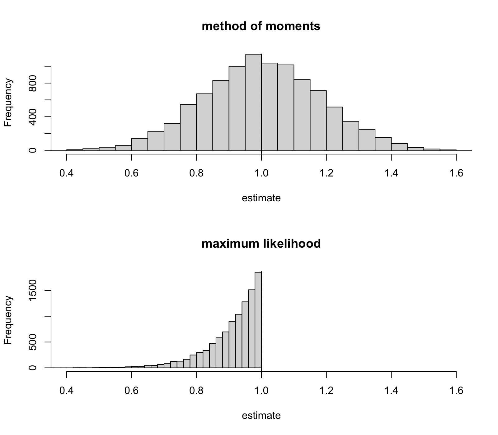
Figure 6.1 shows that the first two guesses were right, and that the third guess is wrong for most people. The top histogram is a symmetric, bell-shaped histogram, centred around the dashed line: the estimator $2\bar{X}$ is unbiased. The bell-shape is expected, since it is an average and by the central limit theorem (theorem A.15), averages are asymptotically normal. (We will learn more about this result in lecture 12.) The histogram for the maximum likelihood estimator is much narrower, and is shifted to the left of the dashed line. This indicates a bias $-1/11$. The histogram is not bell-shaped at all: no simulated estimates are above $1$, since the maximum of a sample from $\text{Uniform}(0,\theta)$ can never be above $\theta$ and the estimates are converging to this boundary. This shows that not every estimator has a bell-shaped sampling distribution: the central limit theorem only applies to averages and does not apply to the maximum. We will see this histogram again in lecture 13, where the uniform model will be used as a counterexample to the general theory.

In lecture 9 we will vary the sample size and will see the histograms getting tighter around the truth.

Just type the commands you see in this solution in your own R session, to make sure you understand what they do.