Lecture 30 Do the Standard Tests Work?

The data set sleep, built into R, contains the amount of extra sleep (in hours) for ten patients, when treated with two different drugs. The two measurements for each patient are paired, and thus we can combine the two measurements into one pair difference as shown in the third row of table 29.1 and then perform a one-sample $t$-test. The command t.test can be used to perform the test which example 29.2 performed manually. Before you try the command, look at the ten differences and consider whether the mean of these differences is positive, and whether the two-sided $p$-value is likely to be less than $0.05$.

Every number in the output is a number we have seen before: the statistic $t=\sqrt{10}\cdot 1.58/1.23=4.06$ is compared with the $t_{9}$ distribution, the $p$-value $0.0028$ is $2\,\mathbb{P}(T\geq 4.06)$ as in definition 20.8, and the interval $[0.70,2.46]$ is the $t$-interval from example 25.4.

The Bayesian answer. We can model the differences as $N(\theta,\sigma^{2})$. To apply proposition 26.6 we pretend that $\sigma$ is known and equal to $s=1.23$, i.e. we ignore the uncertainty in $\sigma$ as in a $z$-test; a prior distribution on $\sigma$ is beyond the scope of this module. Here we assume that the prior distribution is $N(0,10^{2})$. This prior is large enough to be overridden by ten observations. Before we execute the code, predict the posterior probability of $H_{0}\colon\theta\leq 0$: is it larger or smaller than the one-sided $p$-value $0.0014$, output by t.test with alternative = "greater" (see the script R/S30-sleep.R to compute the probability)?

The posterior distribution is $N(1.578,0.389^{2})$, and the probability $\mathbb{P}(\theta\leq 0\mskip 1.0mu|\mskip 1.0mud)$ is $2.5\cdot 10^{-5}$, as found in example 28.5. The final line, the one-sided $p$-value of the $z$-test with $\sigma=s$ assumed known, coincides with the posterior probability $\mathbb{P}(\theta\leq 0\mskip 1.0mu|\mskip 1.0mud)$ to two significant figures, as discussed in section 28.3 for the case of nearly flat prior. The $t$-test’s $p$-value is sixty times larger, reflecting the fact that the $t_{9}$ tail is heavier than the normal tail. This is the cost of not knowing $\sigma$. The middle line of the output answers a question which cannot be answered by the $p$-value: what is the posterior probability that the effect is larger than one hour of sleep? The answer is $0.93$.

A test at level $0.05$ has a $5\%$ chance of rejecting a true null hypothesis, which is harmless for one test but not when many tests are run and only the significant ones are reported. We simulate twenty $t$-tests, each on a sample of size $20$ from $N(0,1)$, so that every null hypothesis is true. By exercise 20.4 each $p$-value is uniform on $(0,1)$ under $H_{0}$. Before you run the code, predict how many of the twenty $p$-values will be less than or equal to $0.05$.

The expected count is one, and this study happened to produce none. The number which matters is the family-wise error rate, the probability that a study of twenty tests reports at least one false discovery. Since the tests are independent, the exact value is $1-0.95^{20}$. Predict it, then check by simulation over $2000$ studies.

Nearly two studies in three would find a significant result for nothing. This can happen either by testing twenty hypotheses at once, or by testing one hypothesis twenty times. The following function simulates a study where a sample of size $100$ is tested after every ten observations, and the procedure is continued until $p<0.05$: this is the case of the researcher who “collects a few more data points and looks again”. Before you try the function, predict the rejection rate for this procedure under $H_{0}$.

Ten looks at the same data raise the type I error rate from $5\%$ to $21\%$: each single test has level $0.05$, but the procedure formed by choosing when to stop does not, and the reported $p$-value does not know how it was chosen.

The solution to this problem is to adjust the significance level. The two most common corrections are named here for reference, but I won’t test your knowledge of these corrections in the exam. The Bonferroni correction is very simple: it just rejects $p<\alpha/m$, so that the family-wise error rate is at most $\alpha$. This method is very conservative. The Benjamini–Hochberg procedure controls the false discovery rate, i.e. the expected proportion of false rejections, by sorting the $p$-values in order $p_{(1)}\leq\dots\leq p_{(m)}$, and then finding the largest $i$ such that $p_{(i)}\leq\alpha i/m$. The $i$ smallest $p$-values are then rejected. The p.adjust function can be used to perform either correction, and returns the adjusted $p$-values for comparison with $\alpha$. The following box contains a script for a study with $200$ tests, $180$ with a true null hypothesis and $20$ with a real effect $\theta=0.8$. The lines are in random order, so you will need to arrange them to form a working script before you can try the code.

As in lectures 12 and 24, all names must be defined before they are used: n, m and theta must come first, effect depends on theta, the seed for the random draw in the sapply line must be set before the line itself, and the three tables can be given in any order. The command table can be used to cross-classify the decision with the truth. This will give the $2\times 2$ table from lecture 20. Before you try the reconstructed script, predict the number of false discoveries among the $180$ true null hypotheses in the first table, and predict which of the two methods, Bonferroni or Benjamini–Hochberg, will result in more of the $20$ real effects being retained.

Without correction there are $30$ discoveries, of which $10$ are false: one in three of the reported findings is wrong, despite all tests being performed correctly. The Bonferroni method eliminates all ten false discoveries, but also $14$ of the $20$ real effects. The Benjamini–Hochberg method also eliminates all ten false discoveries but manages to keep $17$ of the real effects: the guarantee is weaker, but the method finds many more results. Figure 30.1, generated by the script R/S30-forking.R, shows the $40$ smallest $p$-values and their rank.

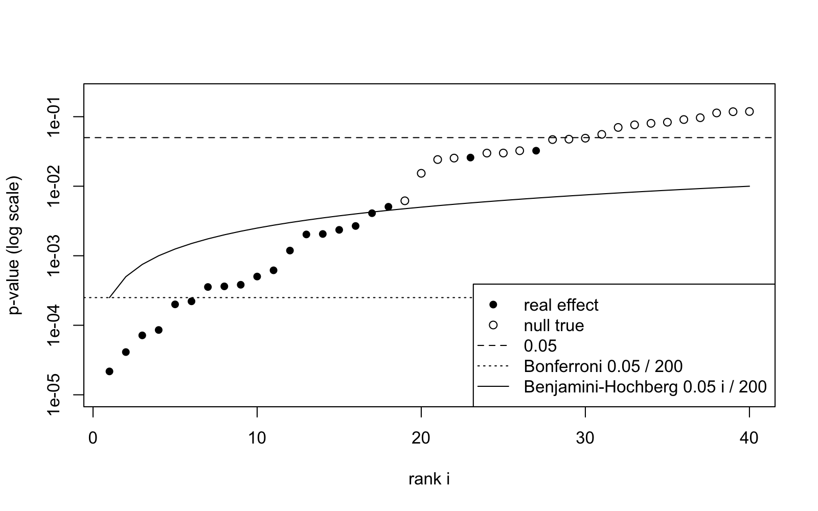
In the figure only six of the real effects are below the Bonferroni line, which does not move with the rank; the Benjamini–Hochberg line rises with $i$, and the last point which is below, the seventeenth, is just before the open circles start at rank $19$.

Every test in table 29.1 assumes that the data are normally distributed. In lecture 12 we have seen that for distributions with heavy tails the central limit theorem takes effect only slowly, and section 17.5 lists further situations in which large-sample approximations are unreliable. We now test the $t$-test for contaminated normal data, i.e. data which consist of $N(\theta,1)$ with probability $0.95$ and $N(\theta,100)$ with probability $0.05$. This could, for example, happen if one in twenty of the measurements is made using a faulty instrument. The resulting distribution is still symmetric around $\theta$ and has variance $5.95$. Before you try the code, consider the following questions: at $n=20$ and level $0.05$, does the size of the $t$-test stay close to $0.05$? What happens to the power of the test at $\theta=0.5$?

The function decide also performs the Wilcoxon signed-rank test, which uses only signs and ranks of the data and assumes symmetry instead of normality. This test is not part of the module under consideration here, but is included for comparison. The first column of the table shows that the size of the $t$-test is preserved under contamination, and in fact decreases to $0.033$: a single ‘wild’ observation has the effect of inflating $S$ more than $\bar{X}$ would, and thus the test statistic is reduced. The power columns tell a different story: for $\theta=1$ the $t$-test on clean data rejects $99\%$ of the samples, whereas the $t$-test on contaminated data rejects only $70\%$ of them. In contrast, the Wilcoxon test, which does not lose much power for clean data, still retains $94\%$. The $t$-test is not lying about the null hypothesis, but is failing to detect the effects present in the data. Figure 30.2, generated by the script R/S30-stress.R, shows the three power curves as a function of the grid of alternatives.

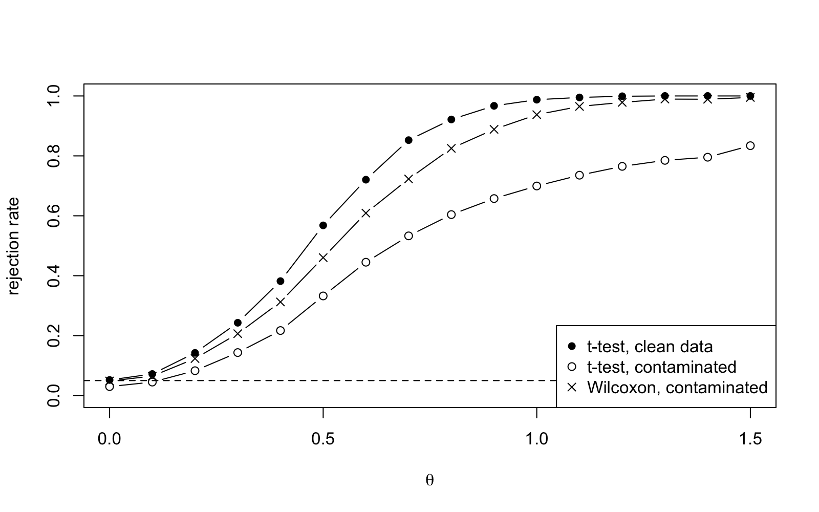
The contaminated $t$-test has the correct size but the wrong power curve; if the contamination was asymmetric, the size would change as well. The moral of the story, as in lecture 24, is that when we are not sure about the model, we should simulate using a plausible alternative model, and should consider both columns of the table.

Seed the generator with your student ID. First repeat the Bayesian analysis of the sleep data with the priors $N(0,1)$ and $N(2,0.5^{2})$ and in two sentences state the change in the posterior probability of $\theta\leq 0$. Then modify the function peek to test every five observations and estimate the rejection rate for $H_{0}$ from $2000$ runs. Compare the estimated rate with $0.206$. Finally, repeat the stress test with $n=50$ and a contamination probability of $0.1$ and create a table of sizes and powers for the test. Write a short paragraph about whether a larger sample size would improve the $t$-test in this example.

Before the next session, you must first understand the commands used in this session. Type in the commands yourself, and make sure that you get the same results as shown in the text.