Lecture 21 EM in R

Throughout, the parameter is the vector $\theta=(\pi,\mu_{1},\mu_{2})$ and the common standard deviation $\sigma$ is known. The E step of example 19.4 computes the responsibilities $\gamma_{i}$, the M step computes the updates (19.2), and both involve only vector arithmetic. The function dnorm is also used to compute the normal density. We also need to compute the observed-data log-likelihood $\ell$. By theorem 19.2, this must increase.

We first test our function on the data from example 19.4. For this we use the five observations $x=(0,1,5,6,7)$ where $\sigma=1$ and initial value $\theta_{0}=(1/2,2,4)$. The results of one iteration of the algorithm are then compared to the responsibilities and iterate $\theta_{1}$ and to the two values for the log-likelihood computed by hand.

Everything agrees with the hand computation ($\mu_{2,1}$ differs in the last digit because the example rounded the intermediate sums), and the last line is the check for exercise 19.3. We now iterate, keeping the parameter and the log-likelihood after each step in a matrix. Before you run the loop, predict the log-likelihood after the second iteration: far above $-9.21$, slightly above it, or equal to it?

The second iteration gains only $0.003$, and after it nothing moves: the responsibilities are so close to $0$ and $1$ that each mean is the mean of its own group, and the iteration has reached its fixed point, a root of the likelihood equation by proposition 19.3.

Convergence in two steps is a consequence of the large difference between the two groups. Here we simulate a sample where the groups overlap. We can simulate such a sample by first randomly choosing a group, using rbinom to get $Z_{i}=1$ with probability $\pi=0.3$. We then simulate the measurements from the normal distribution corresponding to the group, i.e. with means $0$ and $3$ and $\sigma=1$. The command ifelse can be used to choose the correct mean for each observation. The box below contains the complete script for simulation and EM iteration, with lines shuffled (except for the body of the loop). Before you can run the script, you have to arrange these lines into a working script. The loop finishes when the log-likelihood increases by less than $10^{-8}$, as described in section 19.5. The vector ll stores the log-likelihood after each iteration, with the initial value at position $1$.

The rule is the one from lecture 9: each line must come after all lines on which it depends, so the order of lines must be seed, n, z and x, quartiles q, start value, first entry of ll, and then the loop. The start values are chosen such that the weight is at $1/2$ and the two means are at the two quartiles. This is a cheap way to split the sample into two groups. Before you try the script, try to answer the following two questions: How many iterations will the loop take? (In the hand example from lecture, two iterations were needed.) Will the values for the log-likelihood increase by the same amount in each iteration, or differently?

The fixed point $\hat{\theta}=(0.240,0.220,3.076)$ recovers the true group-1 proportion $48/200=0.24$ and the two means to within about two tenths. The loop required $28$ iterations, because the responsibilities of the two means were far away from $0$ and $1$ and because in each iteration the means were only slightly changed. The recorded values are increasing with each iteration, as theorem 19.2 guarantees, but at decreasing rates: $5.0$, then $4.4$, $3.8$, $3.0$, $2.1$, as predicted by the geometric convergence of section 19.5. By proposition 19.3 the fixed point is a root of the likelihood equation. To test this, we can use optim, as shown in lecture 18, by maximising loglik with the same starting values as we used in the EM algorithm. If we use the command hessian = TRUE, we can get the standard errors from section 17.3. (The EM algorithm does not provide the standard errors.)

The two methods agree to four decimal places, and the standard errors say that the fitted weight is $0.240\pm 0.038$, with the smaller group’s mean determined only half as well as the larger group’s. At the fixed point the responsibility of group 1 is a decreasing function of $x$ which equals $1/2$ where $\pi\varphi_{\sigma}(x-\mu_{1})=(1-\pi)\varphi_{\sigma}(x-\mu_{2})$. Before you look at figure 21.1, predict where the crossing lies: at the midpoint $1.65$ of the two fitted means, or above or below this point?

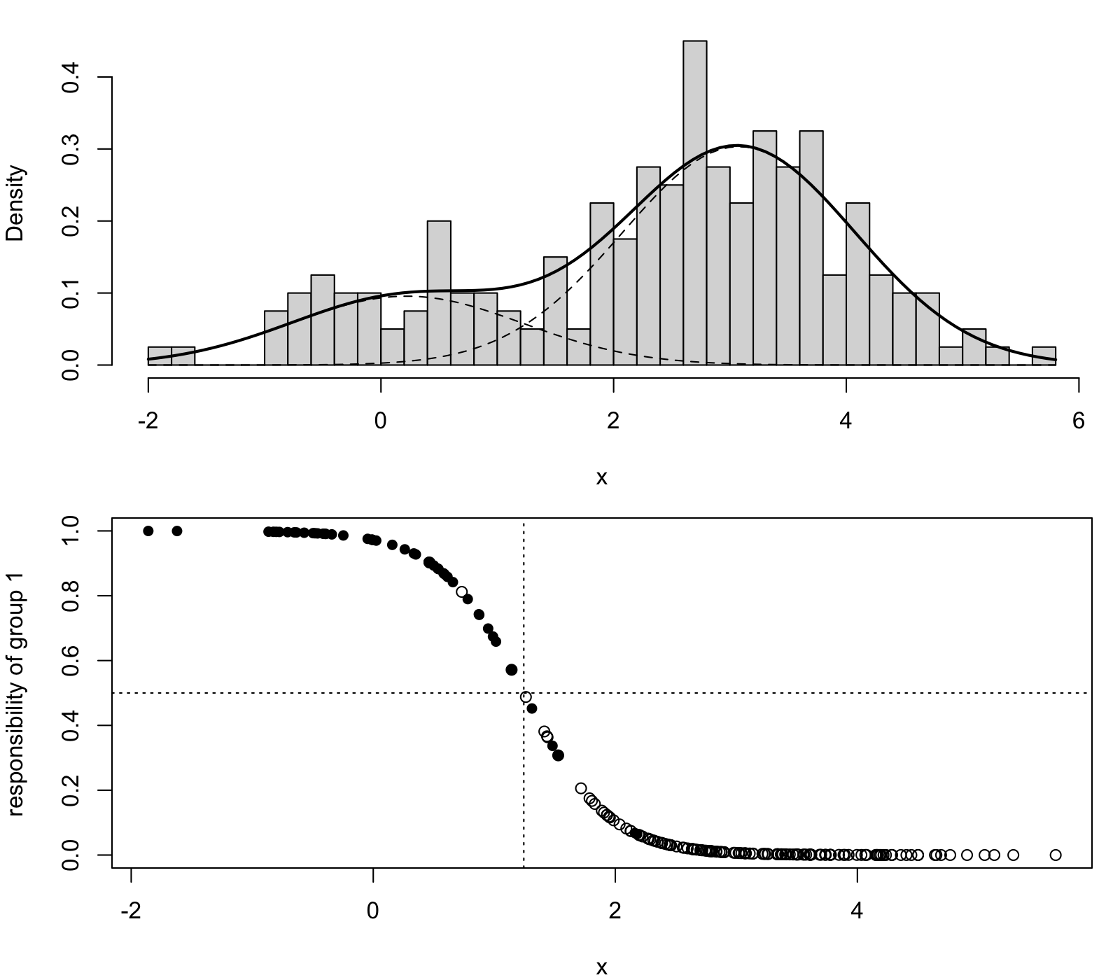
The crossing happens at $1.244$, well below the mid-point $1.648$, since the weights are unequal: an observation which is half-way between the means has three times the probability of being from the larger group. The filled and open circles give the true group of each observation, which cannot be known by EM: the responsibilities agree with the truth when the observations are far away from the crossing point, but between $0.7$ and $1.6$ both types of observations can be found and the group cannot be decided. The top panel is also plotted using the script R/S21-mixture.R; the three functions are given in R/S21-hand.R.

Section 19.5 lists two ways in which a start can lead EM astray; both cases are represented in the sample. The script R/S21-starts.R encapsulates the loop as a function em and then runs this function with four different starts: the quartile start, the start with the two means swapped, the start $(1/2,3,3)$ with both means equal, and the start $(1/2,2.39,2.41)$ with nearly equal means. Before you look at the table, predict the outcome of each row. Where does the start with the swapped means end up? What is the log-likelihood there? What happens to the responsibilities when $\mu_{1}=\mu_{2}$ and thus to the next update?

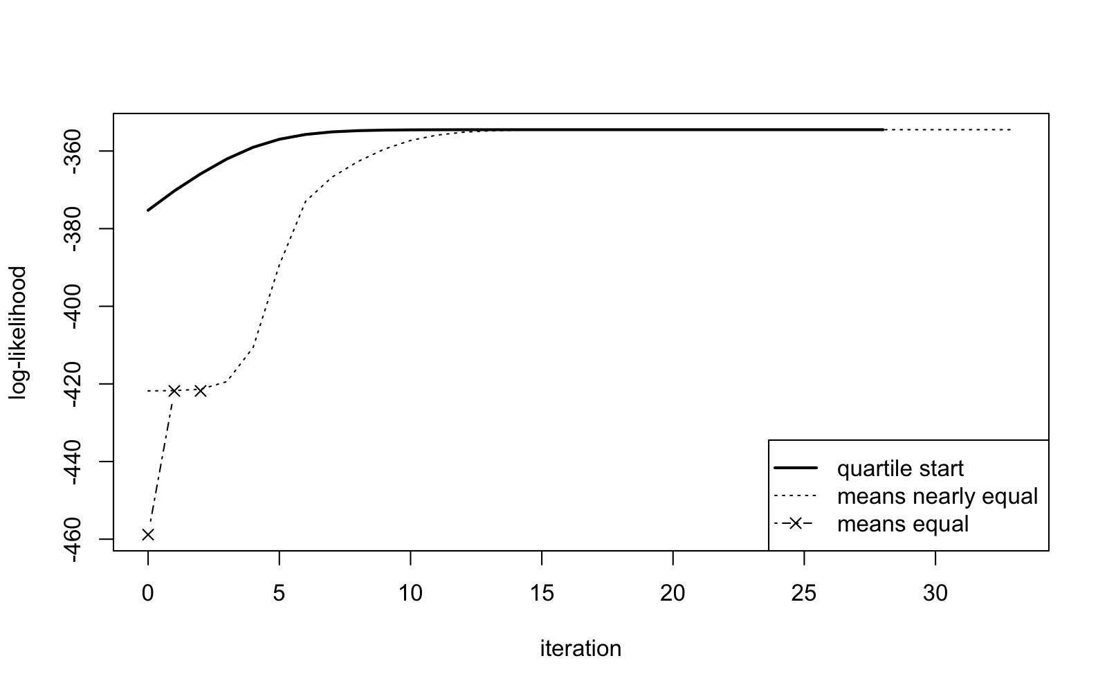
The start with swapped means ends in the mirror image $(0.760,3.076,0.220)$ after the same $28$ iterations and with the same log-likelihood: both parameter values lead to the same density, the model is not identifiable in the sense of definition 4.10 and the choice of labelling in the start determines which of the two maxima we reach. The start with equal parameters is the trap. In this case, with $\mu_{1}=\mu_{2}$, the two normal densities in the responsibility cancel, all $\gamma_{i}$ are equal to $\pi$ and the M step sets both means equal to the sample mean while leaving the weight unchanged; another step does not change anything and the loop stops after two iterations at $(1/2,2.3915,2.3915)$, effectively a single normal distribution, with a log-likelihood $67$ below the maximum. Theorem 19.2 is not violated: the log-likelihood did not decrease but failed to increase. The resulting resting point is a root of the likelihood equation, by proposition 19.3, but a saddle point instead of a maximum and thus EM will not be able to distinguish between the two. The nearly equal start shows that the trap is narrow: the iteration moves away from the saddle point and then climbs to the maximum, in $33$ iterations, as shown in figure 21.2 for the three traces.

For this model, with known common variance, a grid of hundreds of starting values finds only the two mirror-image maxima and the saddle line $\mu_{1}=\mu_{2}$ as stable solutions. In contrast, if the variances were unknown or if there were three or more components, additional local maxima would occur and the procedure from section 19.5 of starting the EM algorithm with several runs and then choosing the run with the highest observed-data log-likelihood becomes essential. For a two-component mixture, the twelve lines of resp, mstep and loglik are all we need. For serious work there are packages: mclust fits mixtures of this kind, and requireNamespace("mclust", quietly = TRUE) reports whether it is installed. Nothing in this session relies on it.

The following task is in the style of a practical report. The published scripts of this lecture can be used as a starting point. Using your student ID as the seed, choose a weight $\pi$ between $0.2$ and $0.5$, and choose two means which are two to three units apart. Simulate one sample of size $n=300$ from the mixture with $\sigma=1$. Run the EM algorithm with three different starting values (the quartile start and two of your choice) and show the fixed point, log-likelihood and number of iterations for each run in a table. Justify which run you would keep and mention if label switching occurred. Finally, use optim with hessian = TRUE to estimate the standard errors for the kept run. For each parameter, show the estimate, the standard error and the interval $\hat{\theta}\pm 1.96\,\mathop{\mathrm{se}}\nolimits(\hat{\theta})$ from corollary 17.3, in three sentences. For each sentence, state whether the interval contains the value you chose. Plot the responsibilities against the data. Write a short paragraph about how many observations have responsibility values between $0.2$ and $0.8$. Comment on how well-separated the two groups are in your plot. Finally, repeat the whole exercise with the two means only one unit apart, and say in one sentence what changes.

Typing the commands yourself is an important step towards understanding how the R scripts work. Before the next session, please type in the commands from this session, and check that you get the same results as shown in the text.