Lecture 15 Cramer–Rao and Efficiency in R

Our model of choice for this section is $X_{1},\dots,X_{n}$ i.i.d. Poisson with mean $\theta=3$. From example 11.6 we know that the Cramer–Rao bound for an unbiased estimator for $\theta$ is $\theta/n$. The sample mean, $\bar{X}$, is an unbiased estimator for $\theta$ with $\mathop{\mathrm{Var}}\nolimits_{\theta}(\bar{X})=\theta/n$ (see lemma 2.2) and thus, by definition 13.4, is an efficient estimator. We use simulation to verify this claim, using the loop over ns from lecture 9. The command var can be used to compute the sample variance of a vector of estimates, and dividing the bound by this value allows us to estimate the efficiency of the estimator. The full script for this section, with lines intentionally shuffled (except for the function body and the loop which are left as one piece), is given in the following box. Before you can run the script, you will need to arrange the lines yourself.

As in lectures 6 and 9, all names must be defined before they are used: the function, theta and ns come first, v needs length(ns), the seed must be set before the loop, and the table must be created last. Before you try the reconstructed script, make a prediction for the efficiency column. Will all entries be exactly $1$? Can an entry be larger than $1$, despite the fact that theorem 13.2 states that no unbiased estimator can have a variance smaller than the bound?

The empirical variances in the table follow the bound for all sample sizes, and the estimated efficiencies are clustered around $1$ with half of the entries above this value. The following argument shows that this is no contradiction: the statement of the theorem only bounds the true variance $\mathop{\mathrm{Var}}\nolimits_{\theta}(\bar{X})$, whereas the table shows the variance of $10000$ random estimates. The random sample is off the true value by one or two percent in either direction, as shown in lecture 6. An estimated efficiency of $1.017$ means that, within the limits of error of the simulation, the estimator is efficient.

In this section we show that not every unbiased estimator is efficient. As an example, from exercise 13.4 we know that the bias-corrected maximum likelihood estimator $\tilde{\theta}=(n-1)/\sum_{i}X_{i}$ for the exponential rate $\theta$ is unbiased and has variance $\theta^{2}/(n-2)$. On the other hand, the bound from example 11.8 is $\theta^{2}/n$ and thus the efficiency of this estimator is $(n-2)/n$. We can perform a similar analysis as in the previous section, this time for $\tilde{\theta}$ with $\theta=2$: To do this we write a new function (below est_pois in the code) to compute the estimator, keep the loop as before, adjust the range of ns to $5$ to $100$, and replace the bound by theta^2 / ns. The resulting script is R/S15-efficiency.R. Before you can run the script, you need to write down $(n-2)/n$ for $n=5$, $10$, $20$, $50$ and $100$. Considering the simulation error we have observed, for which sample sizes could the simulation be expected to distinguish $\tilde{\theta}$ from an efficient estimator?

For $n=5$, $10$ and $20$ the simulation coincides with the exact efficiencies up to two decimal digits. For $n=50$ and $100$ the difference to $1$ is $4\%$ and $2\%$, comparable to the size of the simulation error. Thus, the last two rows do not give useful results and we would need significantly more than $10000$ repetitions to resolve these results. The loss of efficiency is a constant factor which goes to zero as $n$ increases: $\tilde{\theta}$ is asymptotically efficient in the sense of lecture 17, but not efficient.

Where does the difference come from? The proof of theorem 13.2 in lecture 13 uses the Cauchy–Schwarz inequality between the estimator $T$ and the score $\ell^{\prime}(\theta)$. Dividing through shows that the efficiency of $T$ is given by the squared correlation between $T$ and the score. This equals $1$, if and only if $T-\theta$ is a multiple of the score. For the Poisson sample $\bar{X}-\theta$ equals $\theta/n$ times the score, and thus the correlation is $1$ without any calculation. For the exponential sample $\tilde{\theta}-\theta$ is a function of the score, but not a linear one. The following function computes the estimation error and the score for a given sample of size $n=5$. The command cor can be used to compute the correlation of two vectors. Predict the value of the squared correlation before you run the code.

The squared correlation $0.615$ coincides with the efficiency $3/5$ from the table, up to simulation error. A plot of expo[1, ] against expo[2, ] shows that the $2000$ points lie on a curve instead of on a straight line. The curvature of this curve is evidence that the bound does not account for all of the variance.

Example 13.6 is this week’s counterexample: for $X_{1},\dots,X_{n}$ i.i.d. uniformly distributed on the set $(0,\theta)$, the estimator $(n+1)\max_{i}X_{i}/n$ is unbiased and has variance $\theta^{2}/\bigl{(}n(n+2)\bigr{)}$, whereas the Cramer–Rao formula, using the value $\mathbb{E}_{\theta}\bigl{(}\ell^{\prime}(\theta)^{2}\bigr{)}=1/\theta^{2}$ from example 11.11, would give $\theta^{2}/n$. The following function computes, for the same sample, the bias-corrected maximum and the method of moments estimator $2\bar{X}$, both of which are unbiased. Thus, the variances are what the theorem would be about, if it held. The command apply can be used to apply a function to every row (second argument 1) or column (2) of a matrix, in this case to compute the variance var for each row of estimates. Before you try the code, make a prediction: which of the two columns will be below the column $\theta^{2}/n$? Will the other column be above it?

The variance of $2\bar{X}$ is $\theta^{2}/(3n)$ by exercise 2.2, one third of the formal bound at every $n$. The first column is below the formal bound throughout and falls away from it: at $n=1000$ the variance of the corrected maximum is $10^{-6}$, one thousandth of $\theta^{2}/n$. As in lecture 9, a plot on log-log axes shows the rates. Predict the slopes of the two sets of points and of the dashed line $\theta^{2}/n$.

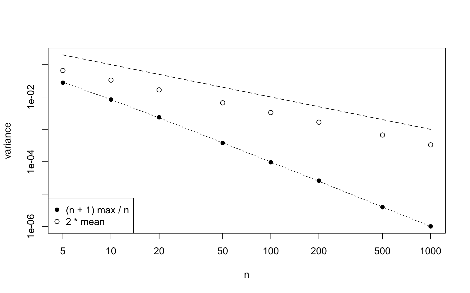
In figure 15.1 the open circles are parallel to the dashed line with slope $-1$, corresponding to the usual rate, and the filled circles follow the dotted line with slope $-2$: figure 9.2 again, with the value $\theta^{2}/n$ added and filled circles placed below it from the first sample size on. Nothing is broken. The regularity conditions of theorem 13.2 are violated by the uniform distribution, since the support of the distribution moves with $\theta$: example 11.11 shows that the score does not have mean zero and that the differentiation under the integral sign used in the proof is not possible. Thus, the value $\theta^{2}/n$ cannot be a bound and indeed it is a formula used outside its domain of validity, and an estimator with variance smaller than this value is called super-efficient. The same failure of regularity is shown in exercise 17.3 to cause the rate $1/n$ of the maximum.

The following task allows you to practice the methods we have learned in this lecture, in a style similar to the practical report. First, you should repeat the study of section 15.1 for the Bernoulli distribution with $\theta=0.3$, where $\bar{X}$ is unbiased and the bound is $\theta(1-\theta)/n$ as shown in example 11.5. Create a table which shows the estimated efficiencies for the sample sizes in ns. Next, consider the sample variance $S^{2}$, computed using var, as an estimator for $\sigma^{2}$ for a normal sample with $\mu=0$ and $\sigma^{2}=1$. The bound $2\sigma^{4}/n$ for this estimator is given in example 14.6. Compute the exact variance of $S^{2}$ using the chi-squared distribution of $(n-1)S^{2}/\sigma^{2}$ from proposition A.3. Compare the exact efficiency of your estimator to the values in the table. Finally, in three sentences, discuss which of the two estimators is efficient, how much less efficient the other one is, and how many repetitions of your simulation would be required to see the less efficient estimator at $n=100$.

Before the next session, you should type the commands used in this session, and should check that you get the same results as the text.