Lecture 24 Power and Size by Simulation

The test we consider today is the one-sided $z$-test from example 20.6, in the numerical setting of the example: we have $n=25$ observations from $N(\theta,\sigma^{2})$ with known $\sigma=2$ and we want to test $H_{0}\colon\theta=10$ against $H_{1}\colon\theta>10$ at level $\alpha=0.05$, i.e. we reject if and only if $\bar{X}>10.658$. By definition 20.4, the power function $\beta(\theta)=\mathbb{P}_{\theta}(\bar{X}>10.658)$ is a probability, and by theorem A.14 we can approximate this probability by the proportion of samples where the test rejects. As in lecture 12, we write a function which, for one run of the test, returns TRUE if the test rejects and FALSE otherwise. We can then use mean to get the proportion of rejections. Before you try the code, predict the value of mean(rejected). Will it be exactly $0.05$? If not, how far away from $0.05$ would it have to be before you would suspect that there might be a mistake in the code?

The rejection rate for $H_{0}$ is $0.0523$. This is the size of the test in the sense of definition 20.5. The value is not exactly $0.05$, and it should not be: as in lecture 12, the estimate has standard deviation $\sqrt{0.05\cdot 0.95/10000}=0.0022$. The last line of the output shows this value. A value between $0.046$ and $0.054$ is what we expect for a correct test. If we get $0.07$, we should suspect that there is an error in the code. We can use the same function to get the rejection rate for any other $\theta$. Predict the three numbers which follow, for the first value of $\theta$ which is less than $\theta_{0}$, and the other two values are the alternatives considered in example 20.6.

At $\theta=9.5$ the test rejects $0.2\%$ of samples: for the composite null hypothesis $H_{0}\colon\theta\leq 10$ the size is attained at the boundary point $\theta_{0}=10$, as remarked after example 20.6. The values $0.344$ and $0.795$ agree with the exact powers $0.346$ and $0.804$ from that example to within simulation error.

A single number is a poor summary of a test, so we consider the power function of a grid of alternatives. We compare the one-sided $z$-test to the two-sided $z$-test from example 20.7, and the one-sided $z$-test for the first $12$ observations. The final test is wasteful, but a legal level $0.05$ test. What is the cost of the waste? The following box contains the full script, with lines in random order (except for the function body). Before you read the rest of this section, try to arrange these lines into a working script.

The rule is as in lectures 9 and 12: all names must be defined before they are used, and the seed must be set before the first random draw. The new function returns a named logical vector of length three, giving the decisions for the three tests. The command replicate then returns a three-row matrix, and rowMeans returns the three rejection rates. The command sapply can then be used to apply this recipe to every value of the grid. Before you try the reconstructed script, predict the row for the two-sided test. Is the rejection rate of the two-sided test at $\theta=9.5$ above or below the rejection rate of the one-sided test? Is the rejection rate at $\theta=11$ above or below? Predict the position of the half-sample test at $\theta=11$, closer to $0.8$ or to $0.5$?

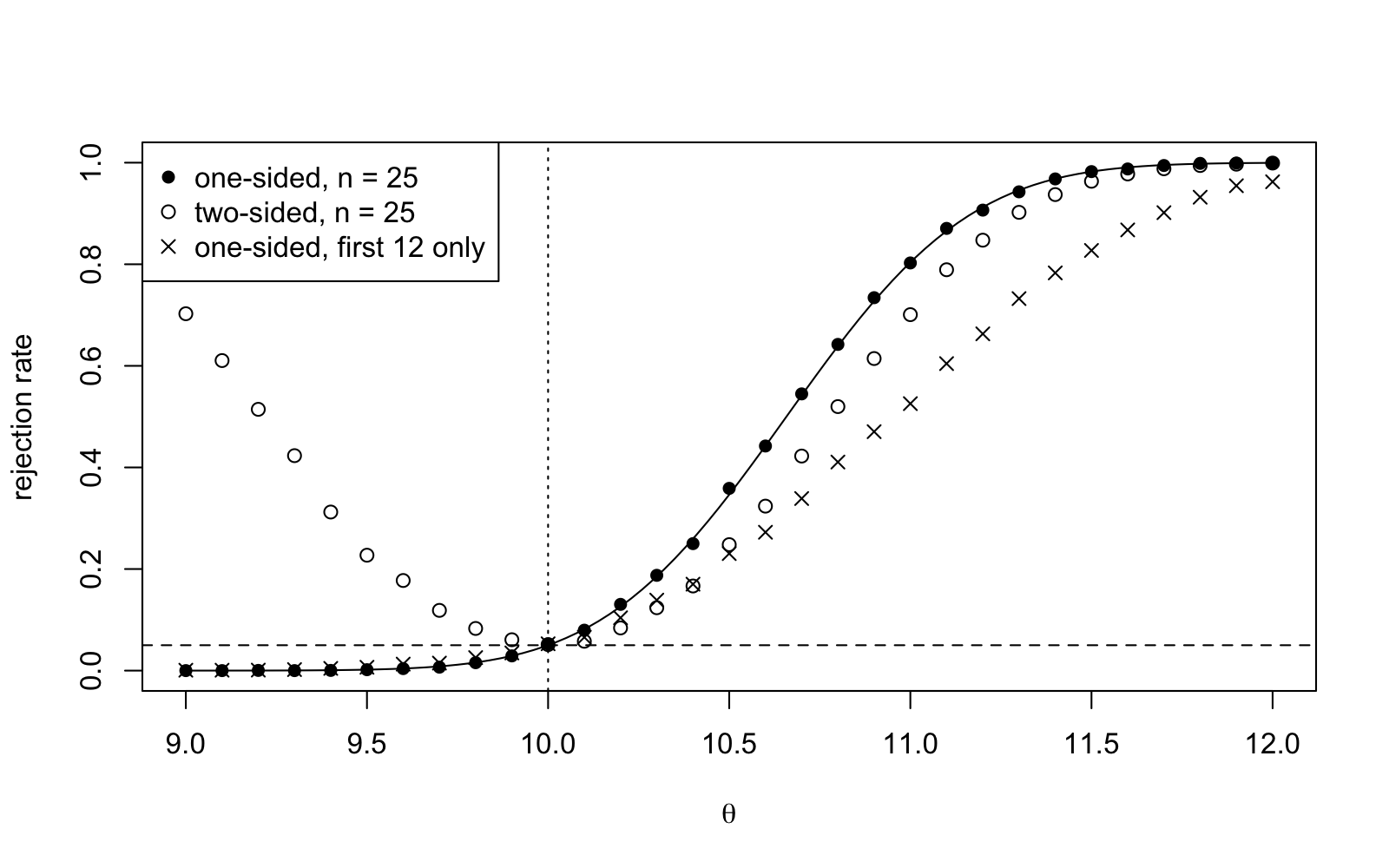
Figure 24.1, produced by the script R/S24-power.R, plots the data for the three rows and the grid. The exact power function (20.2) of the one-sided test is given by the line. All three curves start at $0.05$ for $\theta_{0}=10$ as required for level $0.05$ tests, and the filled circles are on the exact curve at this point. The rest of the plot shows the power of the tests. The two-sided test is always smaller than the one-sided test for $\theta>10$ and is much larger than the one-sided test for $\theta<10$. Thus, neither curve is always larger than the other curve, and this illustrates proposition 22.5. From example 22.3 and proposition 22.4 we know that no level $0.05$ test based on these $25$ observations can reject $\theta=11$ more than $80\%$ of the time, and the crosses indicate what power a poor test would have for this bound: the power at $\theta=11$ decreases from $0.80$ to $0.53$, and this is the cost of having discarded thirteen of the observations.

Assume now that the variance is not known. In this case we cannot perform the $z$-test and we have two parameters, where $H_{0}\colon\theta=10$ is fixed. From exercise 23.1 we know that the likelihood-ratio statistic from lecture 23 is given by

where $S$ is the sample standard deviation, and by Wilks’ theorem (theorem 23.3) the distribution of $W$ under $H_{0}$ converges to a chi-squared distribution with one degree of freedom as $n\to\infty$. In contrast, in the case with known variance from lecture 23, the chi-squared distribution was exact. Here, the approximation will not be exact and we need to determine how well the approximation holds for the $n$ we have. We can simulate $W$ under $H_{0}$ for $n=10$ and $n=100$, using $\sigma=2$ again, and we can reject the hypothesis if $W$ is greater than the critical value $3.841$ of the chi-squared distribution, as if the theorem were exact. Before you try the code, predict the two rejection rates. Will the rate for $n=10$ be above or below $0.05$? Note that the value $S$ in the denominator of $t$ is variable, since $n$ can be small.

The rejection rate for $n=100$ is $0.052$, which is within simulation error of the nominal level. The rejection rate for $n=10$ is $0.075$: the test with nominal level $0.05$ has type I errors half again as often as it should, since $S$ is a noisy estimator for $\sigma$ using only ten observations. The top row of figure 24.2 shows the two histograms, together with the density of the chi-squared distribution. The plot below shows the sorted values of $W$ together with the quantiles of the chi-squared distribution. This is similar to the plot we used in lecture 12 using qqnorm. The command qchisq with ppoints(10000) can be used to get the quantiles. Before you look at figure 24.2, predict the shape of the quantile plot for $n=10$: is the quantile plot on the line, or is it curved above or below the line?

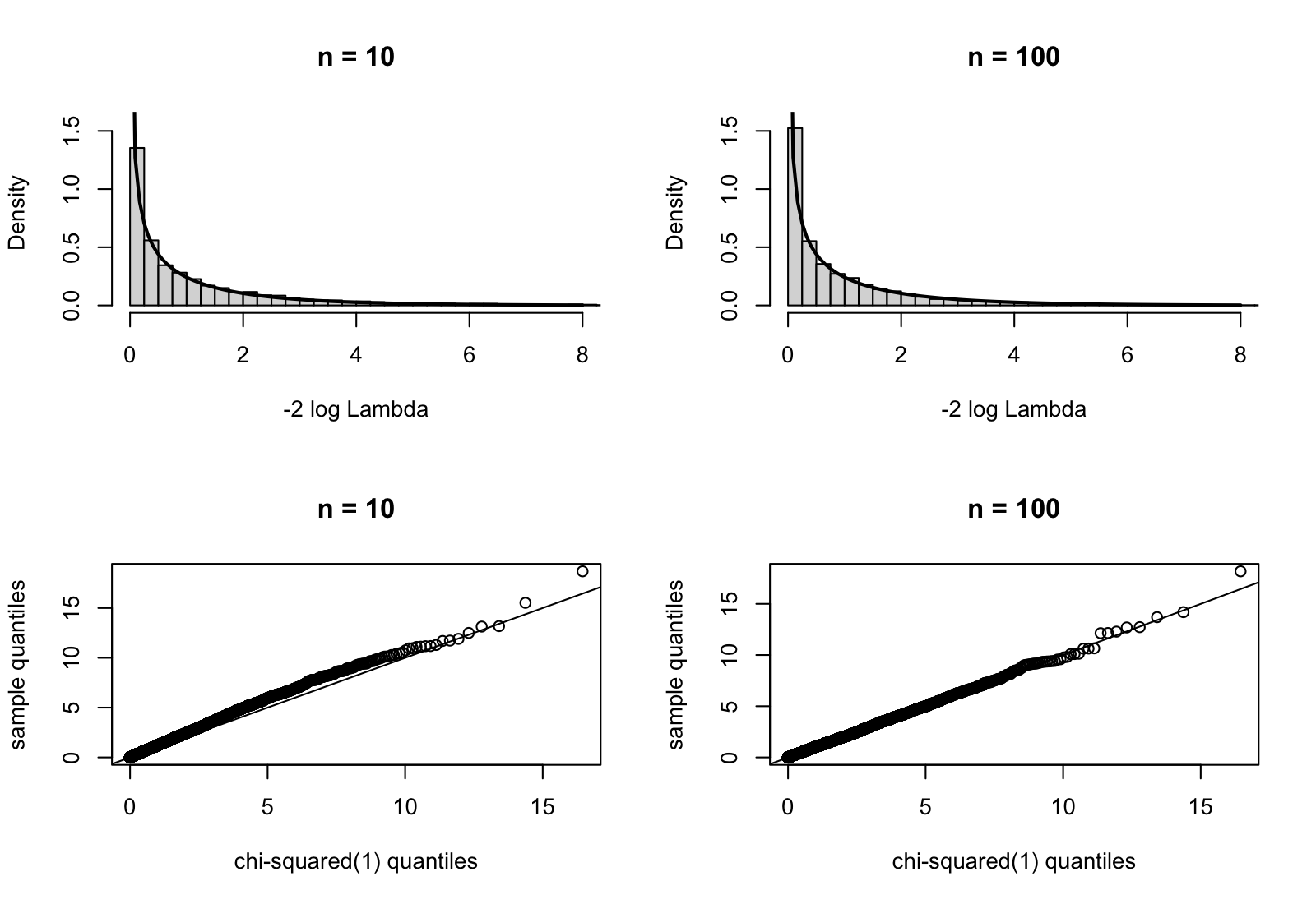
The histograms do not do a good job of showing the difference in sample size, because the density of the chi-squared distribution is unbounded at zero and because most of the mass of the distribution is concentrated in the first few bars. In contrast, the quantile plots show better: for $n=10$ the points start deviating from the line (above) at around $2$, indicating that the upper tail of $W$ is heavier than expected from the limit. For $n=100$ the points stay on the line throughout the plot. The solution to the problem of small $n$ is to use the exact distribution: under $H_{0}$ the test statistic $t$ follows the $t$-distribution with $n-1$ degrees of freedom, and we can reject if $|t|$ exceeds the $0.975$-quantile of this distribution. This is the one-sample $t$-test from lecture 29. Since $W$ is increasing as a function of $t^{2}$, this is equivalent to rejecting if $W$ exceeds the value $n\log\bigl{(}1+t_{0.975,n-1}^{2}/(n-1)\bigr{)}$.

Using the exact threshold $4.50$ instead of $3.84$, the rejection rate for $n=10$ is back to $0.05$ and for $n=100$ the two thresholds are close enough that it does not matter which one is used. An asymptotic level can only be guaranteed in the limit; otherwise, an exact test should be used if available, and if not, a simulation under $H_{0}$ can be used to determine the actual size at a given $n$.

The following task is in the style of a practical report. Set the seed of the random number generator to your student ID and consider the setting from section 24.2, but with sample size $n=10$ instead of $n=25$. Estimate the size of the one-sided $z$-test for $10000$ samples and state whether the estimated size is consistent with $0.05$, within simulation error. Next, estimate the power of the test on the grid seq(9, 13, by = 0.1) and create a plot of the estimated power curve, together with the exact power function from lecture 20. From the plot, determine the smallest $\theta$ at which the power is greater than $0.9$. Finally, consider the test which rejects for large values of the sample median. The critical value must be found first: simulate the median of $10$ observations under $\theta_{0}=10$ and use the $0.95$-quantile of the simulated values to get a test with size $0.05$. (Using the critical value of the $z$-test would lead to a much larger size and comparing the power of two tests with different size is not meaningful.) Estimate the power curve of the calibrated median test and add it to your plot. Write a short paragraph comparing the two power curves, and use example 22.3 to explain why the median test cannot win.

All of this session concerns a single test at a time. The question of what happens when many tests are performed on the same data set and when only the significant tests are reported will be discussed in lecture 30.

Before the next session, type the commands of this session into R, and check that what you get is what the text says you should get.