Lecture 18 Maximum Likelihood in R
This is the R session for week 6. In lectures 16 and 17 we have been concentrating on some mathematical proofs, and in this week we will be considering the resulting theorems in a numerical context: we will find the maximum likelihood estimate for a model where the likelihood equation cannot be solved explicitly, we will learn how to read off the standard errors from the output of the optimiser, and we will use simulation to determine how often the interval from corollary 17.3 contains the truth. The written reference for this session is again appendix B.
18.1 The Log-Likelihood as an R Function
The model of the day is i.i.d. from the gamma distribution with shape and rate , both unknown. Example 4.9 gave the method of moments estimates and , with the plug-in variance, and section 5.3 noted that the likelihood equations have no closed-form solution. We simulate one sample of size with and . The command dgamma with log = TRUE can be used to evaluate the logarithm of the density at every observation, and the sum of these values is . Since the R optimisers minimise, the function returns the negative log-likelihood, and since they hand over all parameters as one vector, it takes the vector par, shape first and rate second.
The true parameter values lead to a much smaller negative log-likelihood than the pair . Here we assume that we know the rate and that we want to estimate the shape parameter . The command optimise can be used to find the minimum of a function of one variable in a given interval, without requiring a starting value. Before you try the command, make a sketch of the negative log-likelihood as a function of on the interval from to . How many dips will there be? Will the minimum lie above or below ?
The estimate is a little above the true value, and the minimum lies below the value where the truth is located. Since both parameters are now unknown, we have to use optim, which minimises a function of a vector, and which requires a starting value. From section 16.4 we know that a good way to find a starting value is to use a simple, consistent estimator. One possible choice for this is the method of moments estimate. Before you try the code, predict whether the maximum likelihood estimates will agree with the method of moments estimates to one decimal place.
The extra argument data = x is passed on to our function. The result fit is a list: fit$par holds the estimates, and , which agree with the start to one decimal place; fit$convergence is if the search finished properly, and any other value means the estimates cannot be trusted; fit$counts records that evaluations were needed. By default optim uses the Nelder–Mead method, which needs no derivatives; appendix B shows the alternative "BFGS".
18.2 Standard Errors from the Observed Information
From theorem 17.1 and the vector version of this result from lecture 17 we know that the MLE is approximately normally distributed with covariance matrix . As in section 17.3, we can replace by the observed information, i.e. the matrix of second derivatives of the negative log-likelihood at the maximum. The optim function can compute this matrix for us if we ask for it explicitly, using hessian = TRUE. The matrix can be inverted using the solve command, the diag command gives the diagonal of this matrix, and the square roots of the diagonal elements are the standard errors. Before you look at the output, predict which of the two standard errors will be larger and by how much.
The table prints the results of a maximum likelihood estimate in an easy to read format. Each row corresponds to one parameter, and shows the parameter estimate, the standard error and the interval from corollary 17.3. Both intervals capture the true parameter values. The standard error for the shape parameter is approximately five times larger than the standard error for the rate parameter, but, since the estimates differ by a similar factor, the two standard errors are comparable relative to the estimates. The final row of the table, computed using the cov2cor function, shows that the two estimates have correlation . It is easy to show that, if we increase the shape and the rate simultaneously, while keeping the mean fixed, the log-likelihood changes only slightly. Thus the data constrains the ratio well, but poorly constrains each parameter individually. This is the problem of a nuisance parameter as discussed in lecture 14.
18.3 Starting Values
The gamma log-likelihood function has only one peak, so the method is forgiving. Before you try the code, make a prediction: what happens if we start with very different values, e.g. with shape and rate ? Will optim still find the maximum? Will it take more than evaluations to find the maximum, when we used the “good” start?
The search reaches the same maximum, up to two decimal places, but it takes more than twice as long and R complains about several warnings and the presence of NaNs (not a number) in the output: the search tried to use negative parameter values where dgamma is not defined. We can prevent this by adding a line at the top of the function which returns Inf if any(par <= 0). This will prevent the optimiser from trying these values. For a “good” start this is not required. The real problem of a poor start is when the likelihood has several local maxima, as in section 5.3. We illustrate this effect using a toy function which is not a model: the logarithm of a two-component normal mixture density, evaluated at , has a local maximum at and a lower local maximum at (see figure 18.1). Which of these two peaks will optimise report for the interval from to , which contains both maxima? Which optim result will you get if you start at and at , respectively? To find the maximum, optim needs to use a different method than the default method, and we can use the BFGS method. Also, we need to tell optimise that we want to find a maximum by using the argument maximum = TRUE.
toy <- function(theta) { log(0.7 * dnorm(theta, mean = 2) + 0.3 * dnorm(theta, mean = -2, sd = 0.7))}curve(toy(x), from = -5, to = 5)optimise(toy, interval = c(-6, 4), maximum = TRUE)$maximumoptim(-3, function(theta) -toy(theta), method = "BFGS")$paroptim(3, function(theta) -toy(theta), method = "BFGS")$par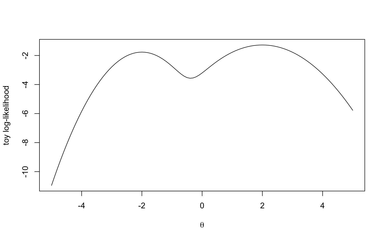
Both optimisers find a local maximum, but neither of them can determine whether this is the global maximum: optim starts at and ends at the first peak it encounters, and optimise assumes that there is only one peak. There is no command which allows us to fix this problem. The only way to avoid this problem is to use some theory and to follow certain habits: always start with a consistent estimator (as we did for the gamma distribution earlier in this lecture), always plot the log-likelihood function (if the number of parameters is one), and always start the optim procedure again to see whether the solution is different.
18.4 Coverage of the Wald Interval
While corollary 17.3 shows that the interval covers the truth with probability approaching , in section 17.5 we have seen that sometimes, for moderate , this is not the case. To verify the claim for the gamma shape and rate, we use simulation in this section, following the approach to coverage introduced in lecture 12. The complete script for our simulation is given in the following box, with the lines shuffled (except for the bodies of the function and of the loop). Before you read the rest of this section, try to do the following: (1) write down the lines in a way which forms a working script, and (2) predict the coverages for : will they be above or below ? Which of the two, shape or rate, will be worse?
data.frame(n = ns, shape = coverage[, 1], rate = coverage[, 2])fit_gamma <- function(n, alpha, beta) { x <- rgamma(n, shape = alpha, rate = beta) V <- mean((x - mean(x))^2) start <- c(mean(x)^2 / V, mean(x) / V) fit <- optim(start, nll, data = x, hessian = TRUE) c(fit$par, sqrt(diag(solve(fit$hessian))))}set.seed(2026)for (i in seq_along(ns)) { res <- replicate(5000, fit_gamma(ns[i], alpha, beta)) lower <- res[1:2, ] - 1.96 * res[3:4, ] upper <- res[1:2, ] + 1.96 * res[3:4, ] coverage[i, 1] <- mean(lower[1, ] <= alpha & alpha <= upper[1, ]) coverage[i, 2] <- mean(lower[2, ] <= beta & beta <= upper[2, ])}alpha <- 2.5coverage <- matrix(0, nrow = length(ns), ncol = 2)ns <- c(20, 100)beta <- 0.5Every name must exist before it is used: the function and the four assignments come first, with coverage after ns; then the seed, then the loop, and the table last. The one new detail is the return value, the two estimates followed by the two standard errors, which replicate stacks as the columns of a matrix; thus res[1:2, ] holds the estimates and res[3:4, ] the standard errors. The script in working order is R/S18-coverage.R; it fits the model times for each sample size, takes a few seconds, and prints the following table.
At both coverages are within simulation error of the nominal , as expected from corollary 17.3. At both coverages are above the nominal level, around : the interval is slightly too wide rather than too narrow. The total hides an imbalance again, and the script also counts for the shape at how many misses are below the truth and how many are above.
Almost three quarters of the misses are below the true shape. Since the standard error increases with the estimate, an underestimated shape will result in a short interval which does not reach the truth, whereas an overestimated shape will result in a long interval which usually still covers the truth. The same mechanism was at work for the exponential rate in lecture 12.
18.5 How Large Is Large?
The results of lectures 16 and 17 hold for large samples, without saying how large is large enough. The sample size needed depends on the shape of the distribution of the data, and we can see this most directly for the sample mean, the simplest estimator we have, where the normal approximation is the central limit theorem (theorem A.15). Tables A.1 and A.2 list three distributions which the lectures do not otherwise use, the negative binomial, the Pareto and the Rayleigh distributions, and these have very different shapes. The command rnbinom can be used to draw from the negative binomial distribution, where size is and prob is in the notation of the table, counting failures before the -th success. The other two distributions cannot be directly generated in base R. Instead we use that, if is uniformly distributed on the interval and is a continuous, strictly increasing distribution function, then has distribution function , since . For the Pareto distribution with we have for , and thus . For the Rayleigh distribution with the square is exponentially distributed with mean , i.e. where is standard exponentially distributed. Before you run the code, sketch the three histograms you expect: which distribution is discrete? Which one starts at ? Which one has the longest tail? Then look up the means and variances in the table.
The empirical means and variances match the values from the table, except for the variance of the Pareto distribution, where is clearly below the table value : the draws have not yet included the large, rare values which contribute much of the variance of this heavy-tailed distribution. The script R/S18-skewed.R continues by computing sample means of draws from each distribution, for example replicate(N, mean(sqrt(2 * rexp(n)))), and by superimposing the normal density from the central limit theorem over the histograms. Before you look at figure 18.2, predict which of the three histograms of means will be furthest from its normal curve.
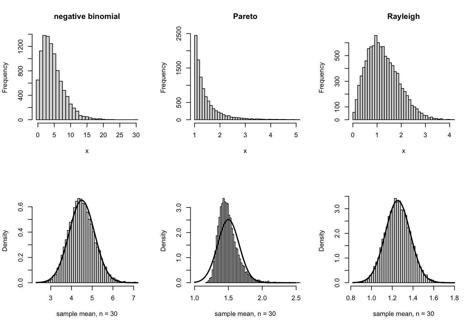
In figure 18.2 thirty observations are enough for the central limit theorem to work well in the first and third columns, but not in the middle column, where the heavy tail leaves the histogram of means visibly skewed. The heavier the tail, the larger must be before the normal approximation can be trusted, and the same holds for the normal approximation of the maximum likelihood estimator behind the standard errors and intervals of this lecture.
18.6 A Task to Take Home
The following task is in the style of a practical report. The published scripts of this lecture can be used as a starting point. Use your student ID to seed the random number generator, and choose your own shape and rate. Simulate one gamma sample of size . Use optim to fit the model by maximum likelihood, starting with estimates from the method of moments. For each parameter, report the estimate, the standard error, and the interval , in three separate sentences. For each interval, state whether the interval contains the value you chose. Estimate the coverage of both intervals when , using replicates. Write a short paragraph about whether you would trust the intervals for this sample size. Finally, fit the normal model with unknown mean and variance, using optim, to a normal sample of size . Check that the estimates match the closed forms from example 5.4, and that the standard error of the mean matches .
Before the next session, you should type the commands used in this session, and should check that you get the same results as the text.
-
•
The written documentation for optim, optimise, solve and the Hessian matrix can be found in appendix B.
-
•
The negative log-likelihood can be represented as an R function for one parameter vector, using the density with log = TRUE. optimise can then be used to minimise this function over an interval for one parameter, and optim can be used to find the minimum for several parameters, starting from a given point. It is important to check fit$convergence to see whether the optimisation was successful.
-
•
If hessian = TRUE, the optimiser returns the observed information matrix. The inverse of this matrix can be used to approximately determine the covariance matrix of the MLE, and the square roots of the diagonal elements can be used to determine the standard errors reported in section 17.3. The results of a fit can be printed in a table which shows the estimates, standard errors and intervals for each parameter.
-
•
A good starting point for the optimisation procedure is to use a consistent estimator, e.g. based on the method of moments. Also, since an optimiser finds a local maximum, it is important to plot the log-likelihood and to re-run the optimisation procedure with a different starting point.
-
•
For the gamma distribution, with shape and rate parameters, the coverage of the Wald interval is slightly above for and close to for , with most of the misses being below the true value. This is caused by small estimates having small standard errors.
-
•
How large a sample the normal approximation needs depends on the shape of the distribution: for sample means of draws the central limit theorem works well for light-tailed data and visibly not yet for heavy-tailed data.