Lecture 3 R Basics and a First Simulation

Appendix B explains how to install R or how to use R on the university computers. Either way, we will end up at the console where we type in commands and R prints the results.

The commands we need to use today are as follows: To construct a list of numbers, called a vector, we can use c. To store a list of numbers under a name, we use the assignment arrow <-. Finally, we can use the built-in functions mean, median and var to summarise a vector.

The [1] at the start of each output line is a position marker, not part of the answer: it gives the index of the first value printed on that line. The assignment itself prints nothing; typing x on its own shows the stored values.

The function var does not use a general convention, but computes the sample variance $S^{2}$ from lecture 2, using the divisor $n-1$. To verify this, we can compute the formula manually, using the fact that arithmetic in R operates on the individual elements of a vector, and that length can be used to determine the number of elements.

The answer coincides with the result of var(x) above, and we now know that R uses the unbiased estimator from lemma 2.3 for variances. Further details about vectors, indexing and arithmetic can be found in appendix B. The appendix also explains how to understand the help page of an unfamiliar command; we will not repeat this information here.

The theory from the last two lectures considers data generated from a model with known true parameter. In this section we will see that we can simulate such data on a computer. The command rnorm can be used to generate a random sample from a normal distribution. The arguments of the command are the sample size and the values for the mean and sd.

Since random draws are different every time, it is often a nuisance to check our work and in a report it would be a disaster if the random numbers changed every time the report was printed. The solution to this problem is the set.seed command: if we call this command with a fixed number, the random-number generator will be set to a fixed state and the same seed will always return the same random numbers.

Any fixed number can be used as the seed. In the practical report, it is a good idea to use a personal number, like your student ID, to seed the random number generator. This way, your report is exactly reproducible, while your dataset is still different from the datasets of your classmates.

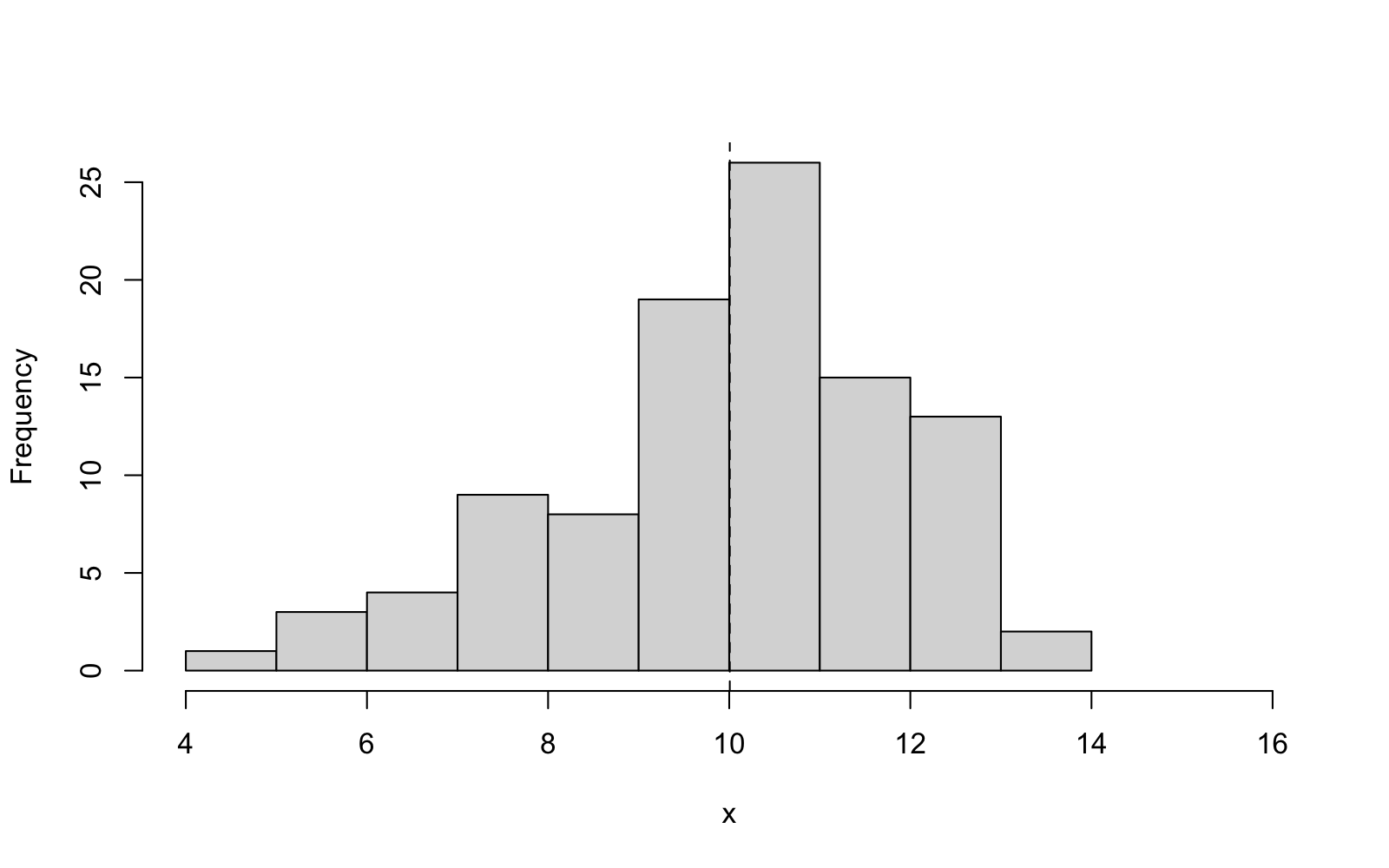
Finally, we can produce a proper sample: $n=100$ observations from the normal distribution with mean $\mu=10$ and variance $\sigma^{2}=4$. The command summary can be used to print the standard descriptive statistics for the sample, and hist can be used to produce a histogram. Finally, abline can be used to add a straight line to an existing plot (in this case, a dashed vertical line at the sample mean).

The summary already tells a plausible story: the sample mean $10.006$ is close to the true mean $10$, and the quartiles are roughly symmetric around the mean. To get a better picture of the sample, we consider the histogram in figure 3.1. We adjust the horizontal range using the xlim argument so that the axis can be compared to the axis in a second figure, below.

In lecture 1 we have discussed the difference between an estimate, a single number computed from data, and an estimator, which is a random variable. We can use simulation to visualise this difference: every call to rnorm below generates a fresh sample of size $n=25$ from the same model as before, and the sample mean of each sample is a fresh realisation of the estimator $\bar{X}$. Before you execute the following three lines of R, make a prediction: will the three printed numbers be equal? If not, how much do you expect the three numbers to be away from the true value $10$?

Three samples, three different estimates, scattered around the true value $10$. The scatter we see here is the sampling distribution, introduced in lecture 1. By repeating the experiment many times, we can map out this distribution. The replicate command can be used to repeat a command a given number of times, and to store the results in a vector. Loops and functions can be used to achieve the same effect (see appendix B). We repeat the experiment $10000$ times, and compare the results to the predictions from lecture 2: From lemma 2.2 we know that the estimator $\bar{X}$ is unbiased, with standard deviation $\sigma/\sqrt{n}=2/\sqrt{25}=0.4$. From theorem 2.7 we know that the mean squared error of the estimator equals the variance $\sigma^{2}/n=4/25=0.16$.

The agreement is striking: the empirical bias is close to zero, the empirical spread $0.4006$ matches the theoretical value $0.4$, and the empirical mean squared error $0.1605$ matches the theoretical value $0.16$. This shows that the theory from lecture 2 is not an abstraction, but accurately predicts the output of the machine with two decimal digits of accuracy.

Finally we draw the histogram of all $10000$ estimates, on the same horizontal axis as figure 3.1 so that the two plots can be compared directly. Before looking at the result, sketch the histogram you expect: where should it be centred, and how wide should it be compared with the data histogram in figure 3.1?

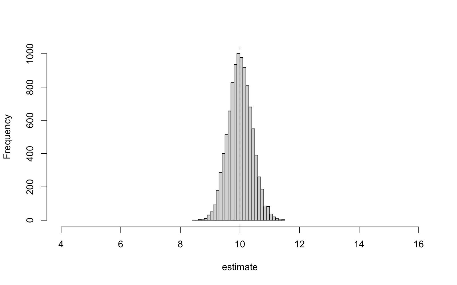
While the data in figure 3.1 are spread out over most of the axis, the simulated estimates form a narrow spike around the truth. This is a consequence of the fact that, by averaging, the estimator has exchanged the spread $\sigma=2$ of an individual observation for the much smaller spread $0.4$ of the estimator. The picture of a histogram of an estimator which is close to the truth is the one we had in mind in lecture 2, when we discussed small bias and small mean squared error. In the next R session, lecture 6, we will use the same simulation setup to compare different estimators. In lecture 9 we will watch the spike get narrower as $n$ increases. This is an example of consistency.

Before the next session, please type in the commands of this session and try to understand the results.