Lecture 27 Confidence Versus Credibility

The interval of the day is the $z$-interval from example 25.3, using the numerical values from the example ($n=16$, $\sigma=2$ are known), so that the $95\%$ interval is $\bar{X}\pm 1.96\cdot 0.5$. By definition 25.1 of the level $0.95$, the random interval contains the fixed value $\theta$ in $95\%$ of all samples. To verify this, we consider $\theta=10$ and compute the interval for $100$ samples. Before you execute the code, answer the following questions: (1) How many of the $100$ intervals will not cover the value $10$? (2) Will all intervals have the same width? (3) Will the misses be clustered or evenly distributed among the 100 samples?

As in lecture 12, covers is a vector of TRUE and FALSE, one for each interval, indicating whether the interval covers the truth. The command mean counts the proportion of TRUE values, which are interpreted as ones and zeros by R. For the example, $95$ out of $100$ intervals cover the truth. The misses are for samples $1$, $29$, $34$, $63$ and $83$. The exact number $95$ is a coincidence, determined by the seed of the random number generator: the number of intervals which cover the truth is binomially distributed with standard deviation $2.2$, so $92$ or $98$ would have been just as unremarkable. The command segments can be used to plot each interval as a horizontal line, and the samples where the interval covers the truth are plotted in grey while the misses are plotted in black.

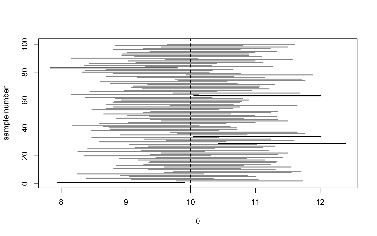
Figure 27.1 illustrates the confidence level of the procedure in a graphical way. The intervals in the figure all have the same width, since the value $\sigma$ is known: the intervals move, while the dashed line stays fixed. The misses are not clustered but are scattered throughout the figure, since the samples are independent. If we had only observed sample $29$, the interval $[10.43,12.39]$ would have been indistinguishable from the others, and there would have been no indication in the data that this was a miss. For this reason, the statement “$\theta$ is in the interval $[10.43,12.39]$ with probability $0.95$” is wrong: the value $10$ is either in the interval or it is not, but in this instance it is not. The probability refers to the procedure, not to the individual values. Before the code is executed, predict the long-run proportion of intervals which cover the truth, and determine the distance from $0.95$ where an error is no longer considered significant.

The long-run coverage is $0.947$. The standard error of this estimate is $\sqrt{0.95\cdot 0.05/10000}=0.002$, so the estimate is about one and a half standard errors below the nominal value $0.95$: this is good agreement, considering the simulation error. The pivot argument in example 25.3 guarantees that this result holds for every value of $\theta$.

We now take the data of example 25.8, $T=37$ successes in $n=100$ Bernoulli trials, and compute two intervals for the success probability $\theta$. The first is the Wald interval $\bar{x}\pm 1.96\sqrt{\bar{x}(1-\bar{x})/n}$ of that example. For the second we treat $\theta$ as random, as in lecture 26: the flat-prior posterior is $\text{Beta}(1+T,\,1+n-T)$ by example 26.5, and the interval between its $2.5\%$ and $97.5\%$ quantiles contains $\theta$ with posterior probability $0.95$; this is the equal-tailed credible interval of lecture 28, and the command qbeta can be used to find the quantiles. Before you run the code, predict whether the credible interval will be wider or narrower than the Wald interval, and whether it will sit to the left or to the right of it.

The two intervals, $[0.275,0.465]$ and $[0.282,0.468]$, coincide to two decimal digits; the credible interval is slightly shifted towards $1/2$, due to the fact that the flat prior adds one success and one failure to the data. The Wald interval states that the recipe used to compute it covers the truth in approximately $95\%$ of samples. It does not make a statement about this particular interval. The credible interval states that, given the observations and the flat prior, the probability that $\theta$ falls between $0.282$ and $0.468$ is $0.95$: the sentence forbidden in the previous section is the correct interpretation in this context, since $\theta$ is a random variable in the Bayesian model. The posterior distribution can be used to answer other questions; the command pbeta can be used to evaluate its distribution function.

The Wald interval itself has posterior probability $0.953$ under the flat prior, and the posterior probability that $\theta$ exceeds $1/2$ is $0.005$. The frequentist interval cannot make a statement about this probability. The final line shows the price of departing from the flat prior: under the informative prior $\text{Beta}(12,3)$, with mean $0.8$ and equivalent sample size $15$, the same data give the credible interval $[0.337,0.517]$. A credible interval always depends on the prior, and numerical agreement with a confidence interval is a property of the flat prior and of the sample size. We will consider this comparison in more detail in lecture 28.

The following picture illustrates the update from lecture 26, where we process the observations one by one. In the example, we simulate $100$ Bernoulli observations with $\theta=0.3$. After $k$ observations, with $s$ successes, the prior distribution with $\text{Beta}(a,b)$ has evolved into the posterior distribution $\text{Beta}(a+s,\,b+k-s)$ with mean $(a+s)/(a+b+k)$. This result was obtained in example 26.5. The box below contains a script for computing the posterior mean of the flat prior after $k=20$ observations. The lines in the box are shuffled, so you will need to sort them into a working script before you can try the code.

As always, names must be defined before they are used, and the seed must be set before the first random draw: theta first, followed by the seed, then rbinom with size = 1 to generate the Bernoulli draws, then cumsum to generate the running total of successes; a, b and k can be placed anywhere before the last line. The script R/S27-posterior.R extends this to handle three priors simultaneously, stored as the rows of a matrix: the flat prior $\text{Beta}(1,1)$, the Jeffreys prior $\text{Beta}(1/2,1/2)$ from example 26.10 and the misplaced prior $\text{Beta}(12,3)$ from the previous section. Before you look at the output of the following code, predict the result: which of the three posterior means will be closest to $0.3$ after five observations? Will you still be able to distinguish between the three posterior means after one hundred observations?

The start of the sequence is bad: the first five observations are all failures and after twenty observations there have been only two successes. The probability of at most two successes in twenty observations is $0.035$ for $\theta=0.3$. For this case, the prediction at $k=5$ is dominated by the flat prior: the posterior mean $0.143$ is closest to $0.3$, since five failures have driven both weak priors below the truth, and the Jeffreys prior is driven lower than the flat prior is. The misplaced prior is still at $0.6$. The two weak priors follow the data and end at $0.14$ and $0.12$, both far below the truth. The misplaced prior, moving from $0.8$ to $0.4$, is the closest of the three at $k=20$: with twenty observations, the data alone is not enough to avoid being misled, but a prior in the correct region helps and a prior in the wrong region does harm. The data does not allow us to infer the correct region. By $k=100$ the two weak priors are indistinguishable at $0.28$ and even the misplaced prior, with an equivalent sample size of $15$, is now mostly aligned with the sample proportion. The script plots the three posterior densities at each stage using curve and dbeta. Before you look at figure 27.2, sketch the panel for $k=5$: which curves are steep, where do they take their peaks and how wide are the curves?

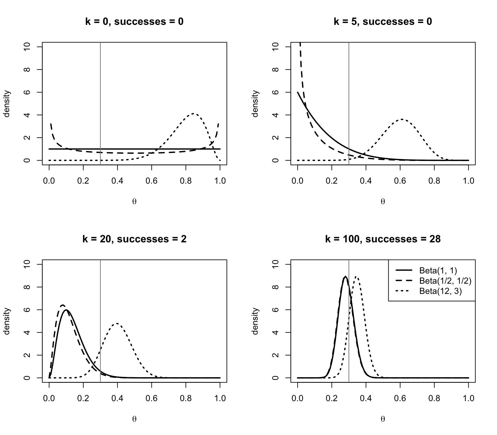
Figure 27.2 summarises the update procedure. At $k=0$ the three curves correspond to the prior distributions from lecture 26. One can see that the Jeffreys prior is not flat. At $k=5$ the two weak posteriors have the largest values at $0$, since no successes have been observed so far, and the informative posterior has not yet significantly changed. At $k=20$ all three posteriors have the form of humps, and the posteriors are narrower than in the previous step: as data are added, the posterior gets sharper, irrespective of the prior distribution. At $k=100$ the two weak posteriors coincide and the informative posterior overlaps these two: this is a consequence of the prior being washed out in example 26.5, and the panel for $k=20$ serves as a reminder that data are needed to achieve this effect.

Repeat the picture in figure 27.1 for the $t$-interval from example 25.4, but with $n=5$, sigma replaced with sd(x) and qnorm(0.975) replaced with qt(0.975, df = 4). The widths of the intervals will change. Estimate how often the intervals miss the target value, and estimate the long-run coverage from $10000$ samples. Repeat the experiment, but this time leaving qnorm(0.975) instead of the $t$ quantile, and comment on your result. Finally, choose a prior mean and an equivalent sample size as in exercise 26.1, use your student ID as the seed for the random number generator, and repeat the posterior sequence of the last section, both with and without the prior. For both cases, determine the first $k$ where the posterior mean is within $0.05$ of the truth.

Type the commands used in this session into R, and check that you get the same results as the text.